# Tutorial
This part is a tutorial on using SCATLAS, for direct users who are about to use SCATLAS to model or readers who are just interested in SCATLAS. As long as they have basic knowledge of supply chain, anyone can easily master the skills of using SCATLAS to build basic supply chain models.
At this point, some readers may be facing urgent business problems and have some experience with SCATLAS, I recommend skipping Chapter 1 and going directly to Chapter 2, "How to Use SCATLAS". For readers who are new to SCATLAS, reading in order is recommended.
# Why use SCATLAS?
The purpose of using SCATLAS is to do supply chain optimization . This chapter will introduce the usage scenarios and main functions of SCATLAS.
# What can SCATLAS do?
SCATLAS can improve the efficiency of supply chain operations, visualize supply chain costs, and assist supply chain management in making multi-scenario decisions. Specifically, it includes warehouse network layout, InventoryPolicies, Products flow optimization, rolling demand planning, and supply chain segmentation strategies.
The following will introduce some of the actual business Scenario and the powerful features of SCATLAS.
# Mock Case 1 Polar Bear
Background of the project:
Company A is a well-known clothing company. Its main products are down jackets, and its sales network is all over China. There are thousands of direct-operated stores and franchised stores across the country. In recent years, the competition among apparel companies has become increasingly fierce, Profit has been declining year by year, and inventory and cost pressures have gradually increased.
Pain point/optimization point: The cost of transportation and warehousing for enterprises is too high. They want to reduce transportation and warehousing costs through the optimization of warehouse network layout, but do not know how to start.
SCATLAS solution: Using the location selection + network optimization algorithm, the warehouse Quantity is reduced from 58 to 25, and the TransportationCost drops by 3.24%, about 100w.
# Mock Case 2 LX Milk
Background of the project:
LX Milk is a well-known dairy company with a sales network all over China. AA, one of its main business units, has 16 factories and can produce 20 kinds of Products, mainly to 55 customers all over the country. The key raw material for these Products - raw milk comes from 14 milk supply places.
The costs within the scope of the project include the ProductionCost of the finished product produced by the factory, milk source-factory, inter-factory transfer, and TransportationCost of the factory-province marketing branches. (Excess raw milk will be made into milk powder, and the cost of discarding is the cost of dusting).
Pain points/optimization points:
LX Milk hopes to optimize the monthly production and sales master plan through software, optimize production and TransportationCost, and improve capacity utilization.
Scala solution:
Through the network optimization (NO) algorithm including the production side, the capacity layout is optimized, the restrictions on the types of products produced in the factory are released, some production lines are closed to increase the capacity utilization rate of the production lines in operation, and the ProductionCost is reduced; ShipmentLane is optimized to reduce the average distribution distance. , reduces the TransportationCost. Optimization results: TotalCost decreased by 5.8%, about 383W yuan; ProductionCost decreased by 3.8%, about 210W yuan; TransportationCost decreased by 21.2%, about 178W yuan.
# How to use SCATLAS
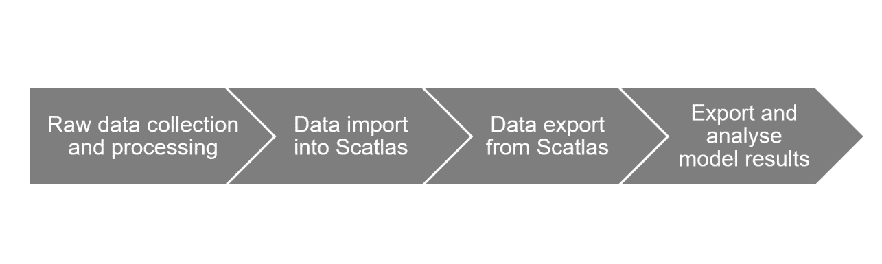
with SCATLAS generally follows the following process:
# Mock Case 1 Polar Bear
# How to reflect the historical situation? Build the Baseline benchmark model.
# Model assumptions
Products : integrated into one kind of products for down jacket
Stores: Stores are integrated according to City and store type
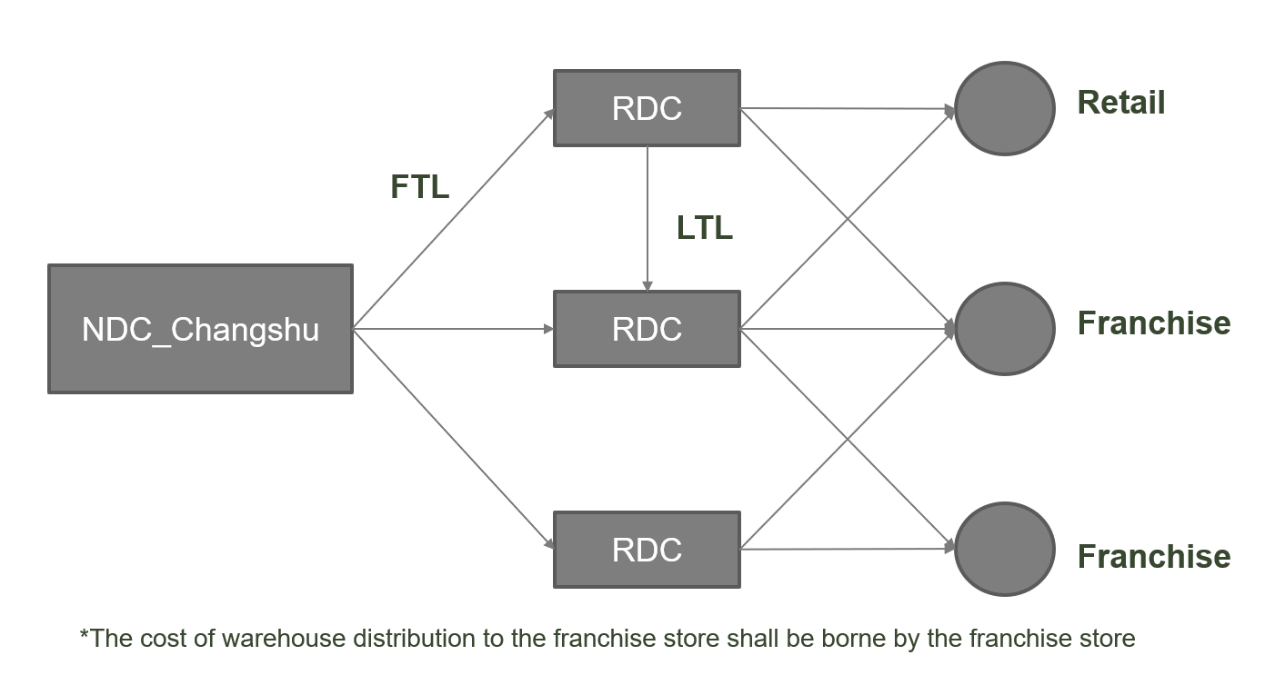
Transportation ModeName: FTL (full vehicle) is used to transport ModeName from the main warehouse to sub-warehouses, and LTL (less-than-truckload) is used to transport ModeName from sub-warehouses to stores.
Missing Shipping Fees: Predicted from Shipping Quotes in Raw Data
# Raw data
# Raw Data Download
Site information
Orders
Shipping route
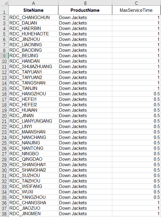
Service Requirements
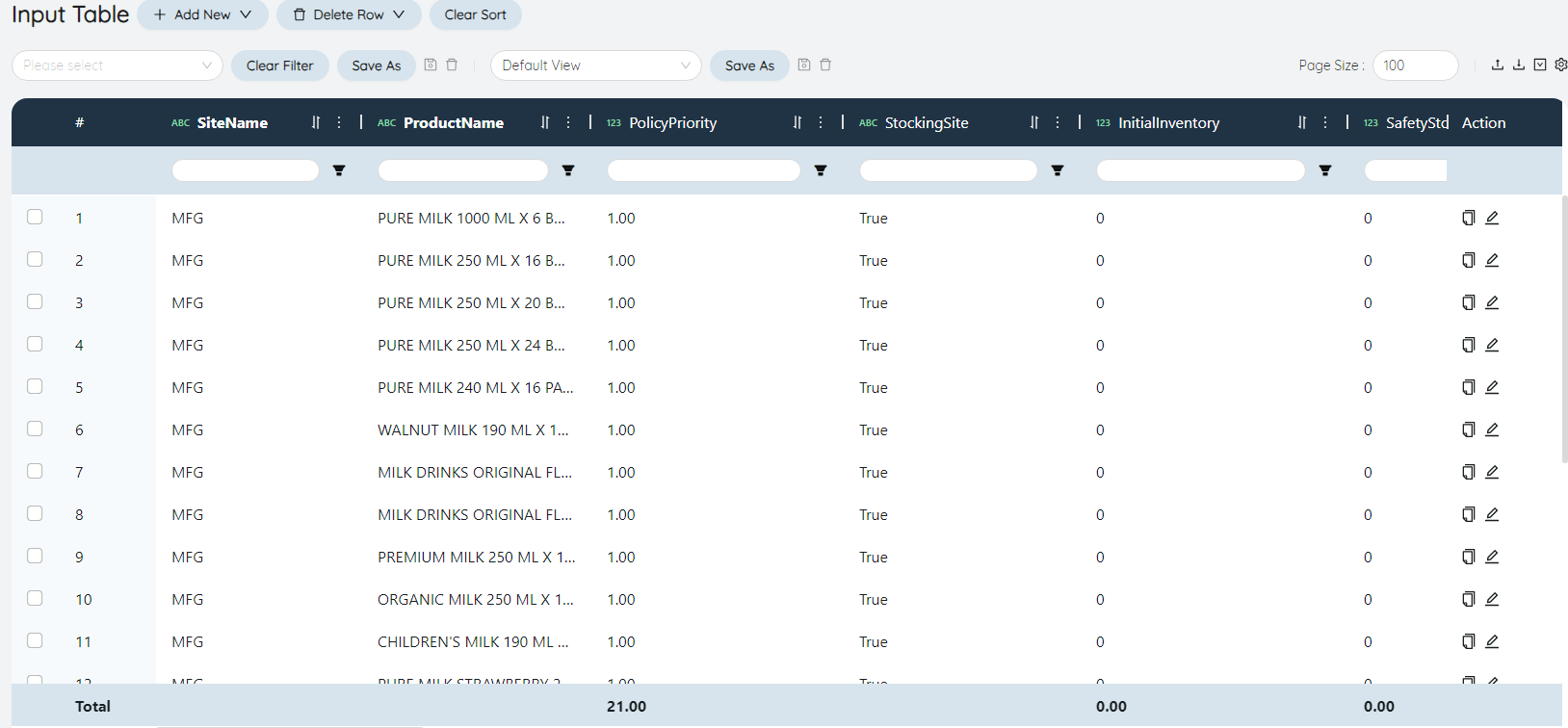
# Model input
Before running the model, the data is entered in tabular form.
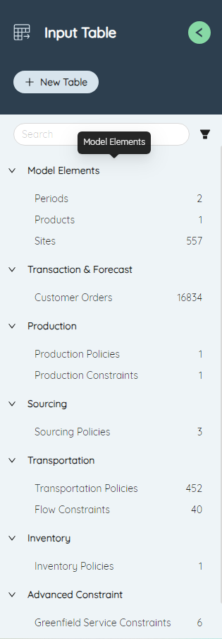
The model input required by different algorithms is different, which is divided into required input and optional input. For example, the required input table of NO is Periods, Products, Sites, CustomerOrders, ProductionPolicies, SourcingPolicies, TransportationPolicies, InventoryPolicies, and GF required The input table only needs Sites, CustomerOrders. Since SCATLAS' data table headers are fixed, the original data needs to be input in a fixed format.
Next, the input table required by the Baseline benchmark model will be introduced, including the meaning of the fields used, the corresponding relationship between the value of the field and the original data.
Click the input form on the left function bar and select the corresponding form to fill in.
Periods
The Periods table represents the SnapshotDate range of the model. There can be only one Periods in the SnapshotDate from the beginning to the end, that is, a single Periods model, or there can be multiple Periods, that is, a multi-periods model.
**Periods Table - Single Periods**
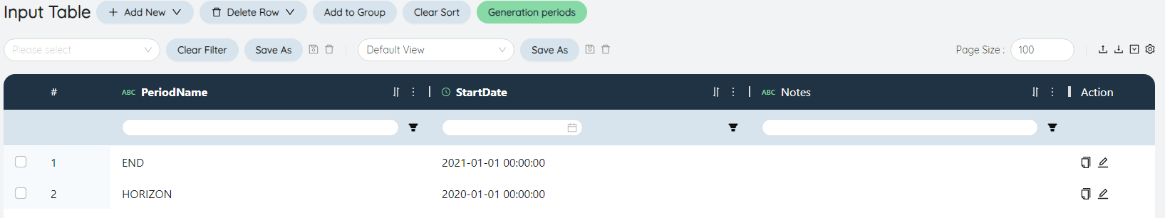
Periods Name
The Name of SnapshotDatePeriods, HORIZON refers to the StartDate of the entire model, END refers to the EndDate of the entire model, and must contain END.
StartDate
HORIZON's StartDate is set to 2020-01-01
END's StartDate is set to 2021-01-01
Products
The Products table records the properties of the Products itself.
Products table
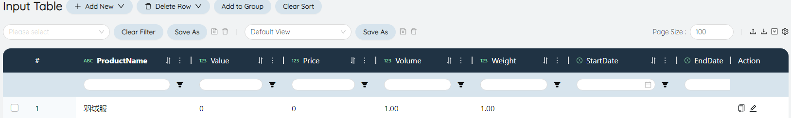
Products Name
Products have been integrated, and there is only one down jacket, so the Products Name only needs to fill in one down jacket.
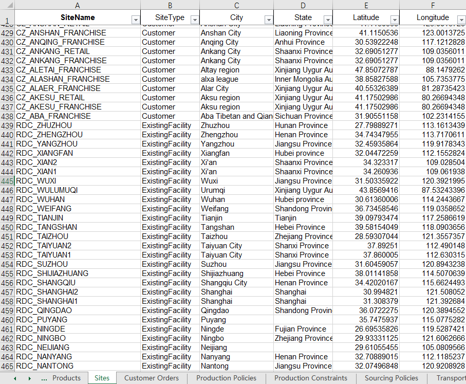
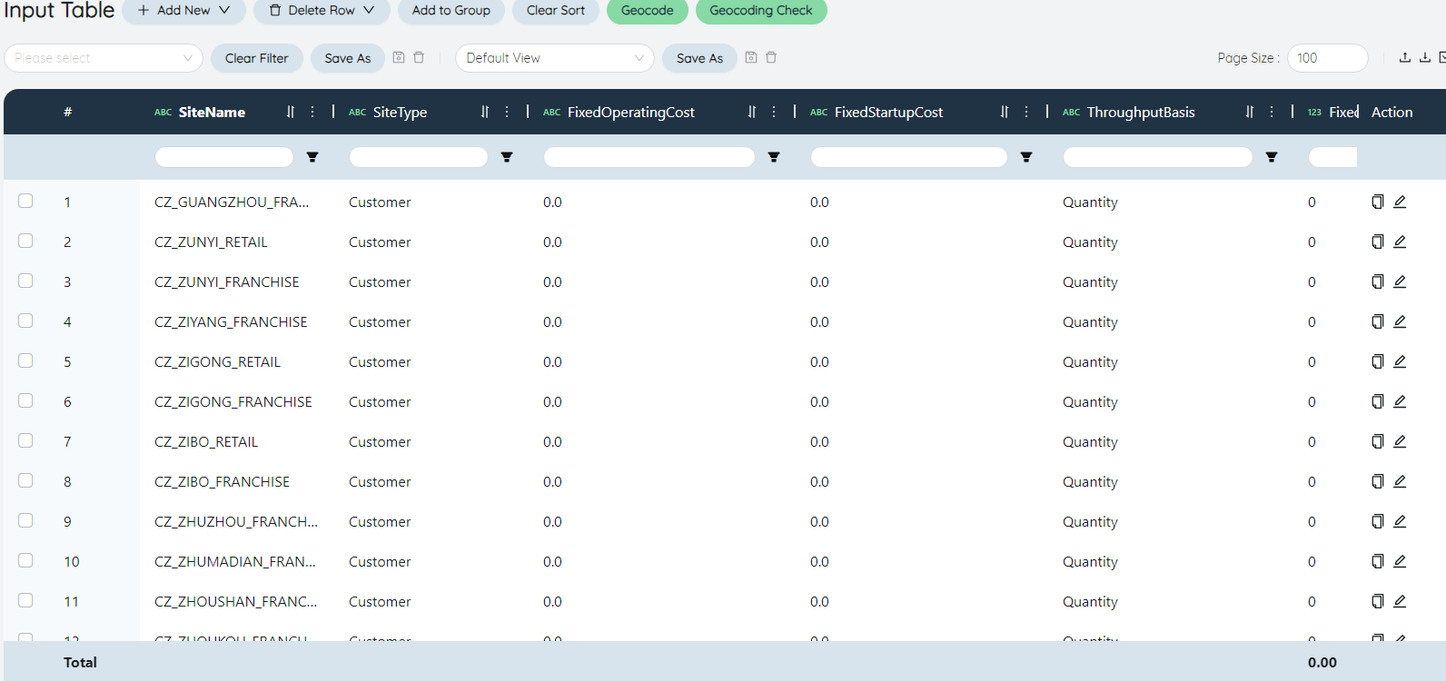
Sites
The Sites table includes total warehouses, sub-warehouses, store locations, and regional information.
Sites table
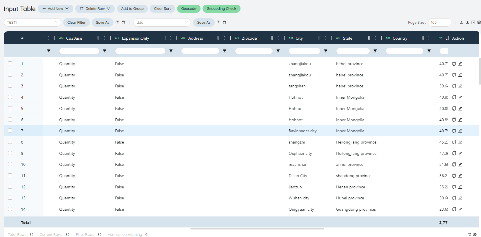
Sites Name
That is, the warehouse name/store name in the original data-warehouse information/store information.
Sites Type
The customer that generates the demand order is the Customer, and the factory/warehouse is the ExistingFacility
City
Original data - warehouse information/city where the warehouse is located in the store information/city where the store is located
Province
Original data - warehouse information/province where the warehouse is located in the store information/province where the store is located
Latitude/Longitude
After filling in the City and Province copies, click the geocoding button above the Sites table to automatically query the Latitude. If there is longitude and latitude in the raw data, it is unnecessary to do so.

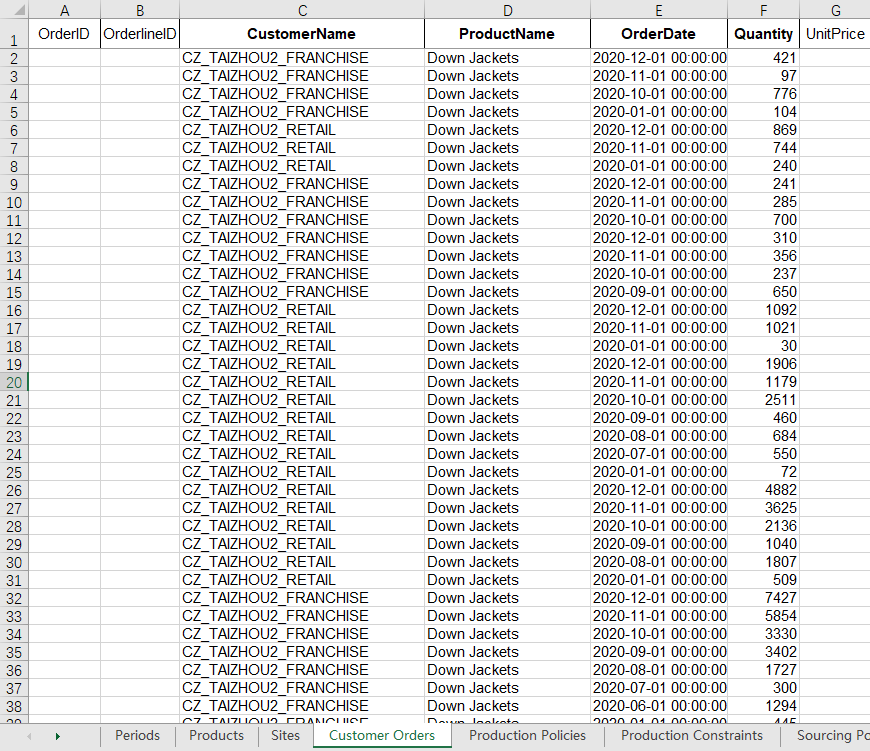
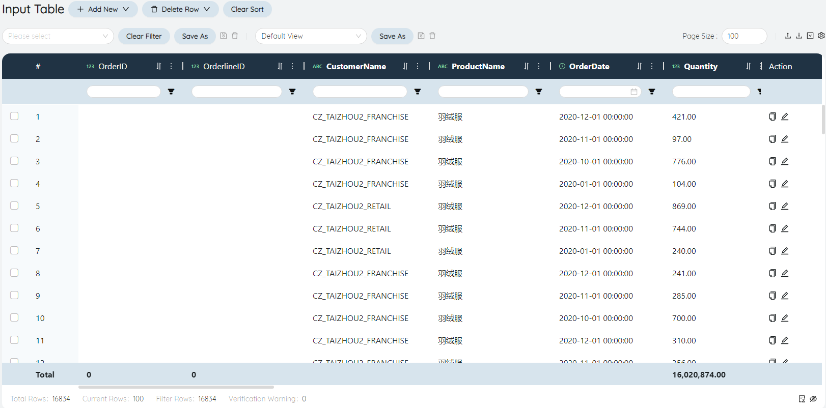
CustomerOrders
The CustomerOrders table records the SnapshotDate and Quantity of each product ordered by each customer, and aggregates the sum of the Quantity according to the store name, product category, and actual arrival month according to the original data-shipping record (sub-warehouse-store). You need to fill in Customer Name, Products Name, OrderDate, and Quantity.
CustomerOrders table
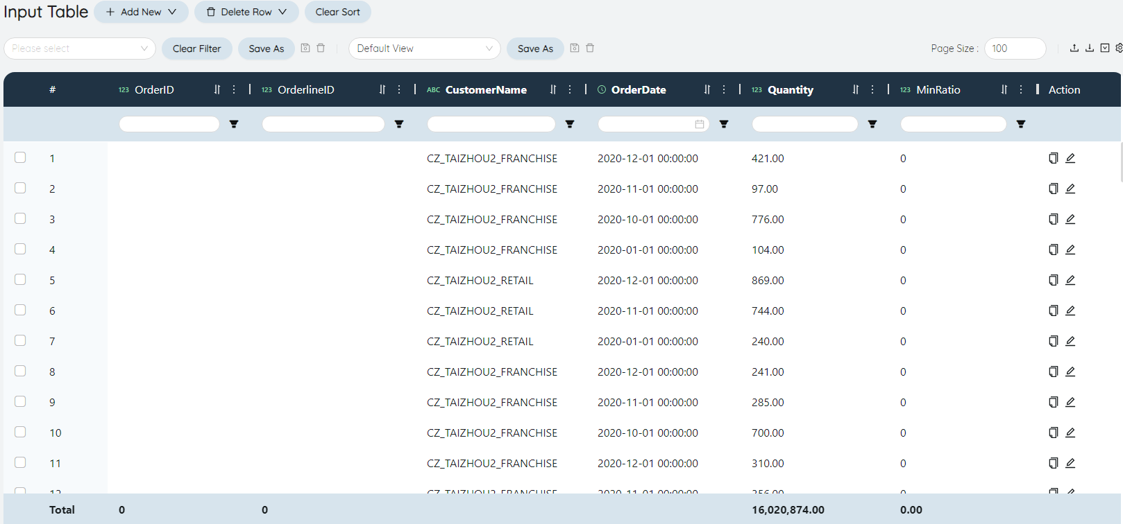
OrderDate
According to the actual arrival month field of the original data-shipping record (sub-warehouse-store), change it to the 1st of the month in 2020
Quantity
The Quantity of each Product purchased by each customer per month.
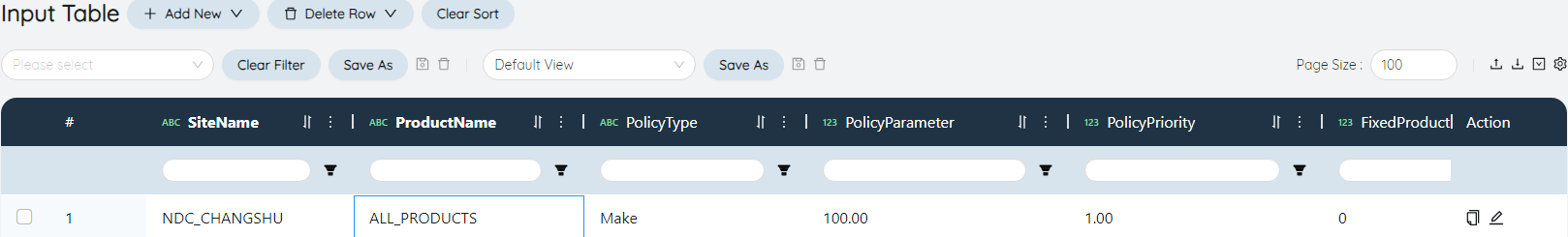
ProductionPolicies
ProductionPolicies records the production source, ProductionCost/Batch/SnapshotDate and other information of Products. Consider the general warehouse as the production source of Products, which can produce all Products. Sites Name and Products Name are required. (Note: Sites and Products appearing in the strategy table need to appear in the model element)
ProductionPolicies table
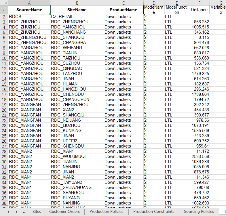
SourcingPolicies
SourcingPolicies record the flow of Products in the supply chain network. Including the purchase of down jackets from the sub-warehouses from the main warehouse, and the purchase of down jackets from the stores from the sub-warehouses. You need to fill in the starting point Name, Sites Name, Products Name. Fill in according to the original data-shipping record (total warehouse-sub-warehouse), original data-shipping record (sub-warehouse-store), one line corresponds to a starting point, a combination of Sites, and Groups of Products, which cannot be repeated.
SourcingPolicies table
TransportationPolicies
The TransportationPolicies table records the transportation ModeName, Distance, TransportationCost and other information of each ShipmentLane. Each row of data corresponds to the SourcingPolicies table, and the information of Transport ModeNameName/function, Distance, VariableTransportationCost, VariableCostBasis, and FixedShipmentCost is added to the starting point/Sites/Products Name. The freight information comes from the freight rate of the whole vehicle and the LTL quotation in the transportation quotation, and the missing freight rate is combined with the mileage forecast.
TransportationPolicies table
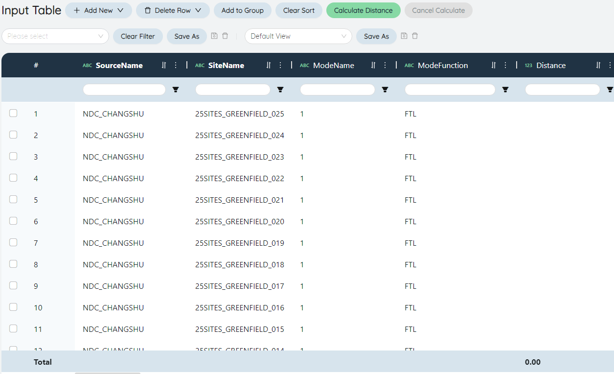
Transport ModeName/Function
The line sent from the main warehouse to the sub-warehouse (the starting point Name is the main warehouse, and the Sites Name is the data row of the sub-warehouse), the transport ModeNameName is 1, and the transport ModeName function is FTL; the line sent from the sub-warehouse to the store (the starting point Name is the sub-warehouse) , Sites Name is the data row of the store) Transportation ModeNameName is 2, and the transportation ModeName function is LTL.
Distance
Click the Distance calculation button above the TransportationPolicies table to automatically query the navigation Distance of each piece of data based on the Latitude in the Sites table.
VariableTransportationCost, VariableCostBasis, FixedShipmentCost
The meaning of VariableTransportationCost changes with VariableCostBasis. For example, VariableCostBasis is QuantityDistance, VariableTransportationCost is 0.13, which means that VariableTransportationCost per kilometer per piece is 0.13 yuan, VariableCostBasis is Quantity, and VariableTransportationCost is 0.26, which means that VariableTransportationCost per piece is 0.26 yuan; For goods (one batch is defaulted to one piece), a fixed additional TransportationCost (such as a starting fee) needs to be paid.
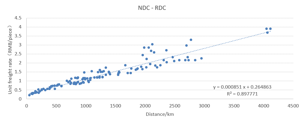
From the total warehouse to the sub-warehouse: VariableTransportationCost fills in the existing part according to the original data-transportation quotation, and VariableCostBasis fills in Quantity; the missing part in the transportation quotation is predicted by linear regression (see the figure below), VariableCostBasis is QuantityDistance, each piece per kilometer VariableTransportationCost of 0.000851 yuan is required, and FixedShipmentCost of 0.264863 yuan per piece.
Total warehouse - sub warehouse freight forecast
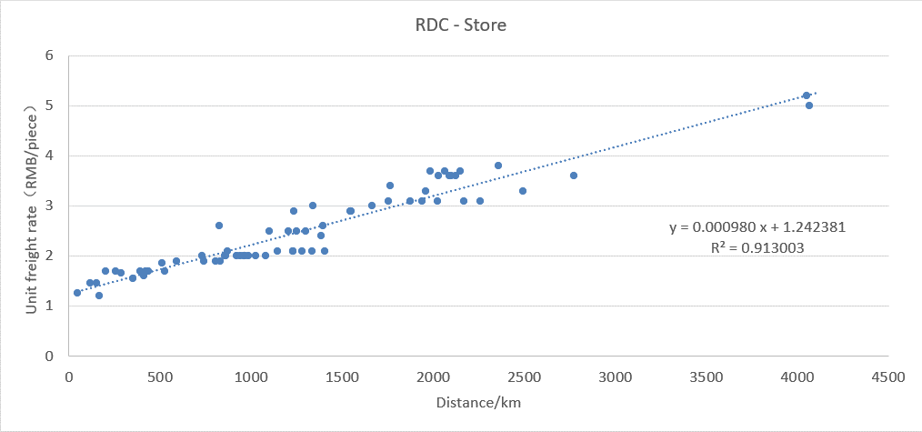
From sub-warehouse to store: According to the LTL quotation in the transportation quotation, it is predicted by linear regression (see the figure below), VariableCostBasis is QuantityDistance, and each piece requires VariableTransportationCost of 0.000980 yuan per kilometer, and FixedShipmentCost of 1.242381 yuan per piece.
Sub-warehouse - store freight forecast
InventoryPolicies
Down jackets are stored in the RDC. Sites Name is the RDCName in the original data-warehouse information.
InventoryPolicies table
# Model output
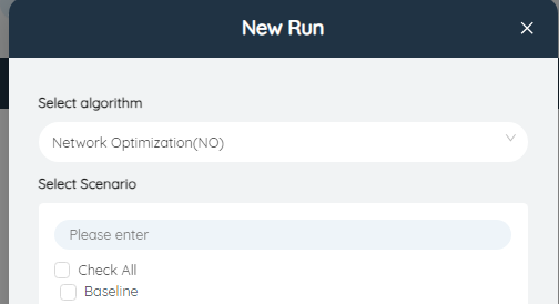
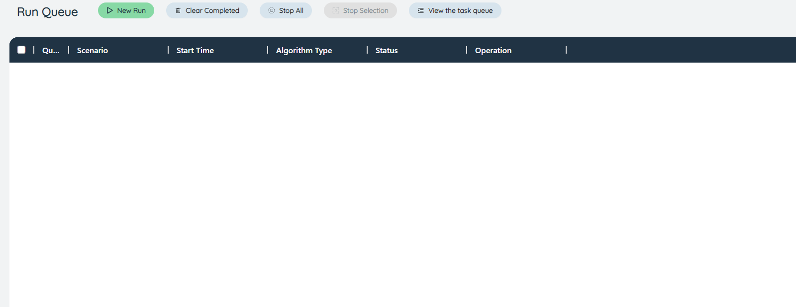
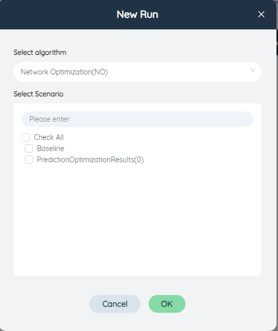
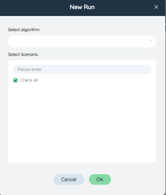
After filling in the input form, click the left function bar to enter the online task list, click Add task, check Baseline, select the algorithm "Network Optimization (NO)", click Add, and the model starts to run.

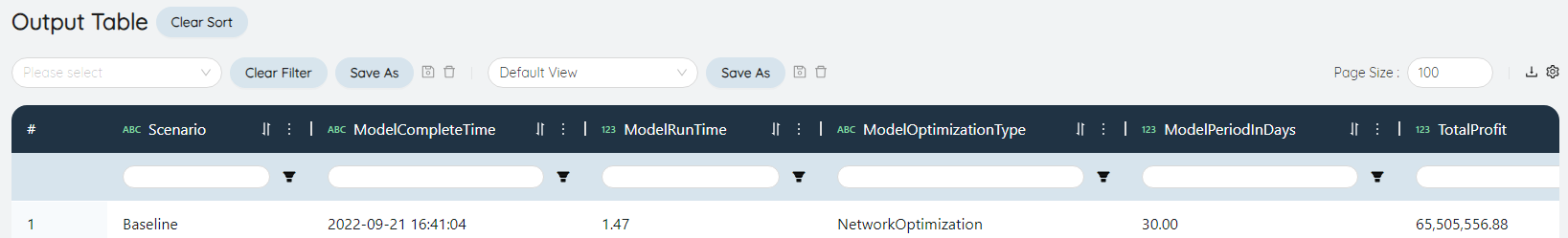
After the operation is successful, click the left function bar and select the corresponding output table to view.
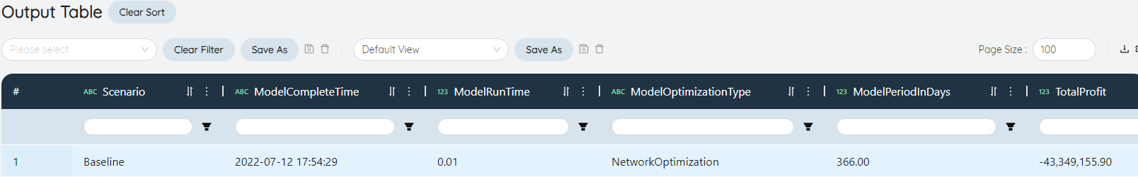
- OutputNetworkSummary
OutputNetworkSummary shows the composition details of TotalCost, total Profit, total Revenue and other information. In this Scenario, TotalCost is equal to TransportationCost, which is about 30,448,304 yuan.
- Network Sites Summary
The network Sites summarizes and displays the optimized Status, ThroughputLevel (outbound flow), and related TotalCost (including inbound transportation, outbound transportation, and warehouse inbound and outbound) of ExistingFacility of each factory/warehouse.
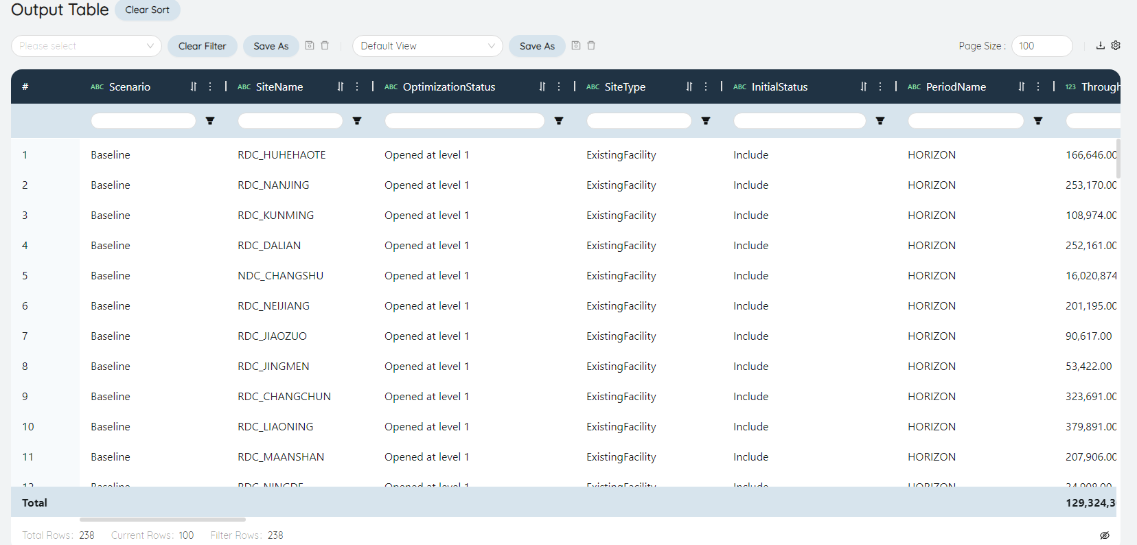
Optimize Status
If an existing facility has a stepped FixedOperatingCost, it means the facility is on the first step.
ThroughputLevel/ThroughputLevel benchmark
Indicates the outbound flow of the facility and the unit of ThroughputLevel (Quantity/Weight/Volume corresponds to /kg/M3).
TotalInboundTransportationCost/Total outbound TransportationCost
Indicates the TransportationCost for shipments entering the facility and the TransportationCost for shipments departing from the facility.
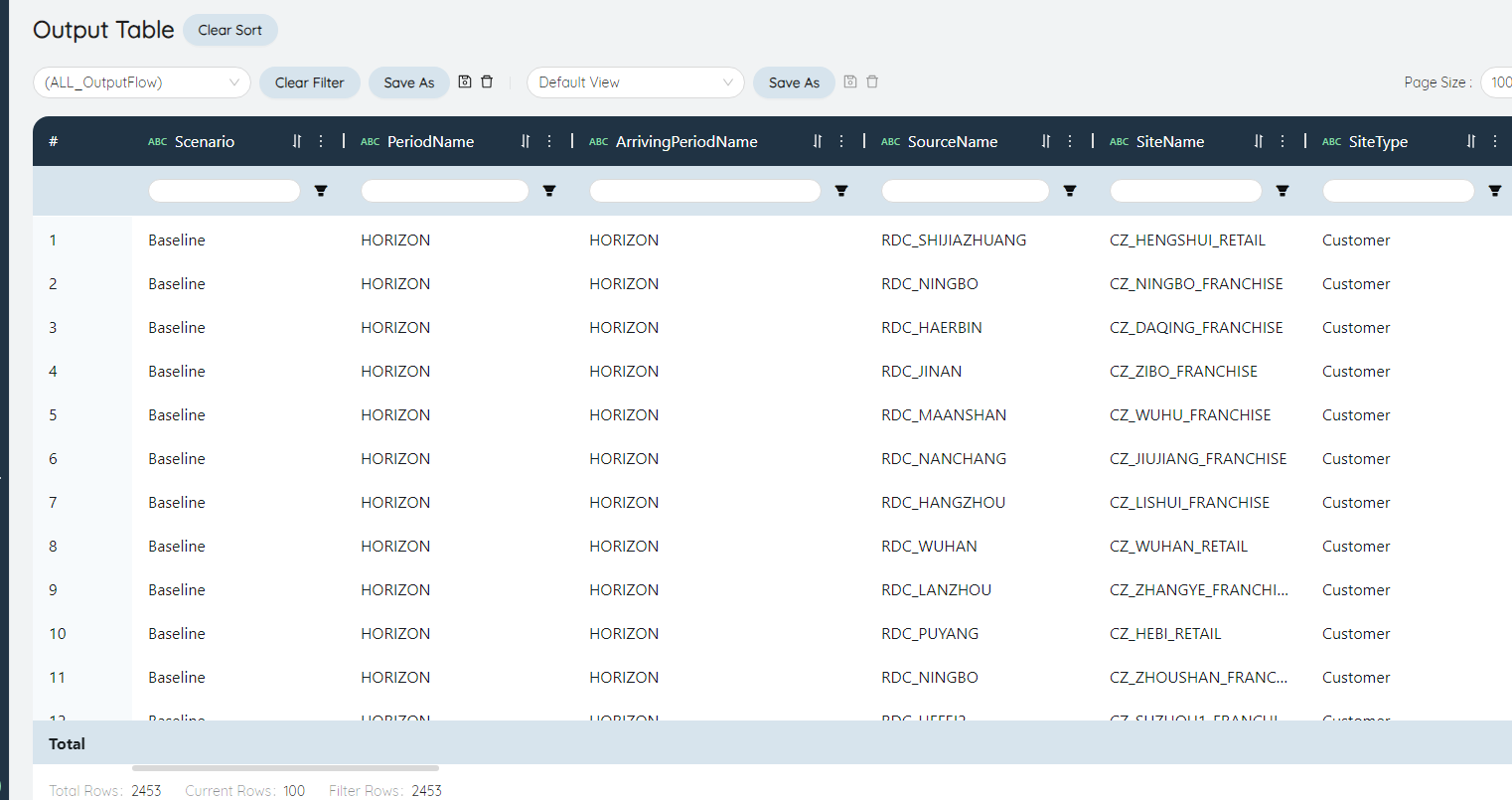
- Flow Details
It shows the traffic, ServiceDistance, ServiceHour, TransportationCost, InTransitInv and other information of each product transported by each mode of transportation on each line.
FlowUnits
Traffic flow is the result calculated by SCATLAS based on the model input table (including policies and restrictions) and aiming at the minimum TotalCost. The sum of FlowUnits is the sum of the Quantity of goods transported by each line, which is equal to the sum of the ThroughputLevel of each facility, which in this Scenario is exactly twice the total outbound flow of the warehouse.
FlowVolume/FlowWeight
Calculated according to the information in the input table Products, equal to FlowUnits*Products unit Volume; FlowUnits*Products unit Weight
ServiceDistance
If there is a Distance in the input table TransportationPolicies, it is equal to this Distance; if not, it is calculated according to the spherical Distance from the start point to the end point and the detour Coefficient.
TotalTransportationCost
Calculated from the input table TransportationPolicies, in this Scenario:
If VariableCostBasis is QuantityDistance, TotalTransportationCost=FlowUnits*(ServiceDistance*VariableTransportationCost+FixedShipmentCost);
If VariableCostBasis is Quantity, TotalTransportationCost=FlowUnits*VariableTransportationCost.
The sum of TotalTransportationCost is the sum of the TransportationCost of each line, which is equal to the TotalTransportationCost of the entire supply chain network.
ServiceHour
Calculated according to ServiceDistance and Options, which is equal to ServiceDistance/default driving speed/24 hours.
# How to optimize warehouse layout? Build the GreenField site selection model.
# Model input
- CustomerOrders
Same as Baseline model without modification
- Sites
Same as Baseline model without modification
- GreenFieldServiceConstraints
Fill in the Sites Name, Distance, and Percentage according to the original data-site selection-service requirements.
Sites Name
Create Groups according to the Sites table, each area corresponds to a Sites Groups SET.
How to create Groups in batches? The operation steps are as follows:

①Click the small cube in the left function bar (see the picture on the right)
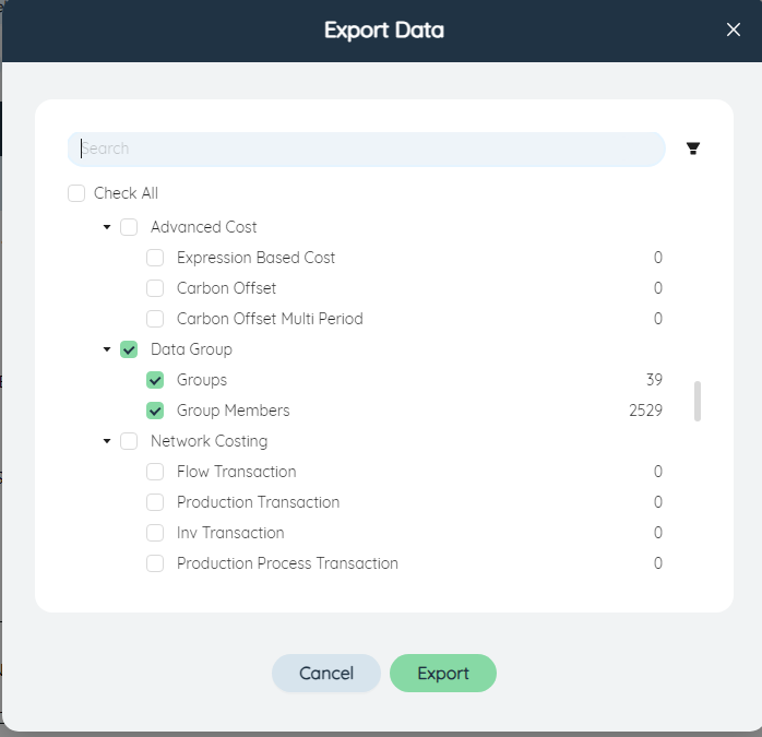
②Select the export data (see the picture on the right)
③ Check the data Groups in the input table, including Groups and Groups members
④Click Export to open the exported Excel
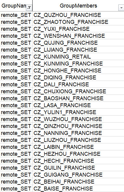
⑤In the Groups sheet, the Groups Type is filled in Set, the Groups entity is filled in Sites (representing the Sites table), and the Groups Name is filled in by area as shown in the figure below

⑥ In the Groups member sheet, the Groups member is the store name in the original data - store information, and the Groups Name fills in the area, and then adds _SET after each area, so that the Groups and Groups members correspond
⑦ Go back to the SCATLAS model interface and click the small cube in the left function bar again
⑧ Select Import Data and import the Excel you just filled in
⑨Select Groups in the left function bar, and see that the Groups corresponding to the seven areas have been established
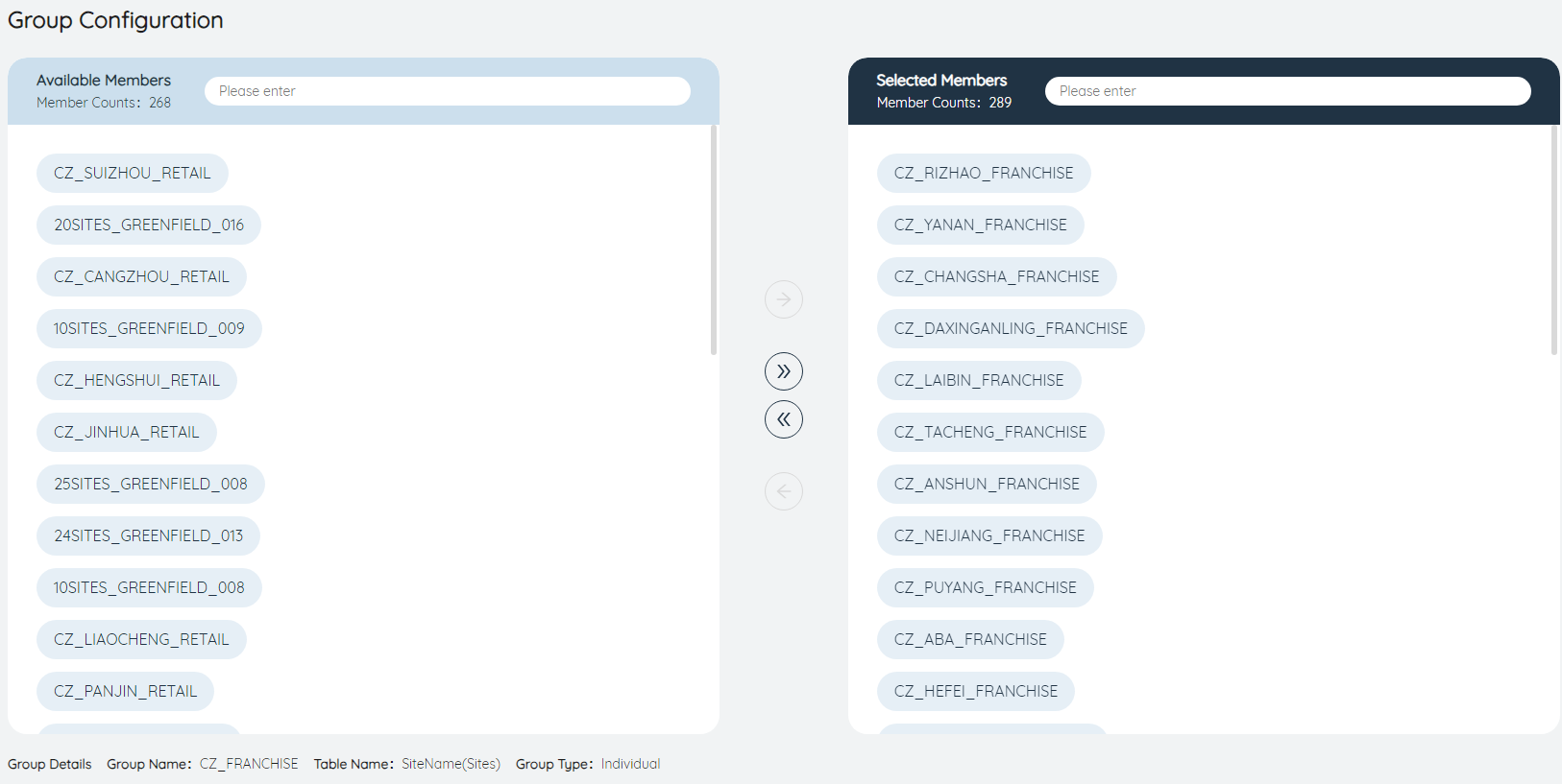
Sites Name can be filled in the Groups name of each Groups.
Distance
Calculated according to the average speed * service SnapshotDate in the original data - site selection - service limit.
Percentage
That is, site selection - the rate of demand fulfillment within service constraints.
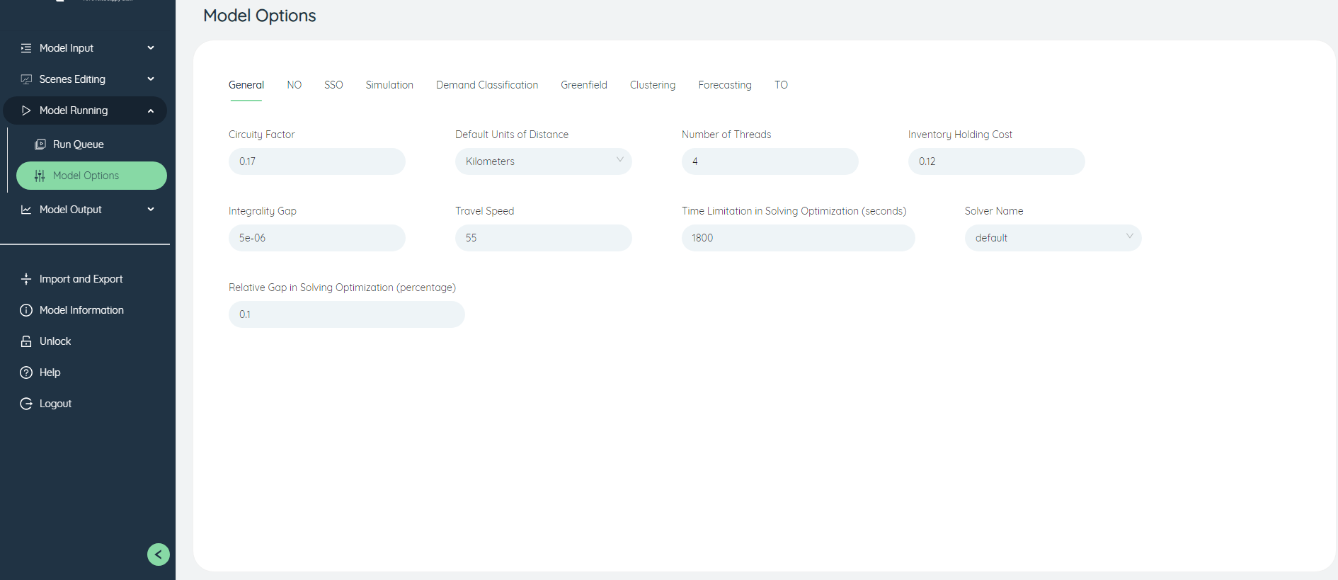
- Options - Site Selection Optimization
Fill in 25 for the site Quantity, and select false considering the existing Sites.
# Model output
After filling in the input form, click the left function bar to enter the online task list, click Add task, select the algorithm "Location Analysis (GF)", click Add, and the model starts to run. The algorithm will find the site selection scheme with the smallest FlowsTimesDistance sent to the client segment under the condition that the site selection service requirements are met.
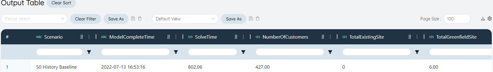
- OutputGreenFieldSummary
The OutputGreenFieldSummary table shows the TotalFlow, total FlowsTimesDistance and weighted ServiceDistance predicted for the new scheme after GreenField is located.
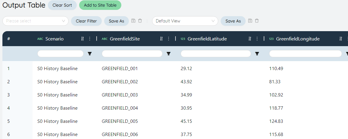
- Site Selection Sites Summary
The locations of the 25 selected Sites and the predicted ThroughputLevel information are displayed.
- OutputGreenFieldServiceSummary
It displays the ServiceDistance predicted by customers with service requirements, and the traffic within the range of Distance, and makes a preliminary evaluation for the feasibility of the solution.

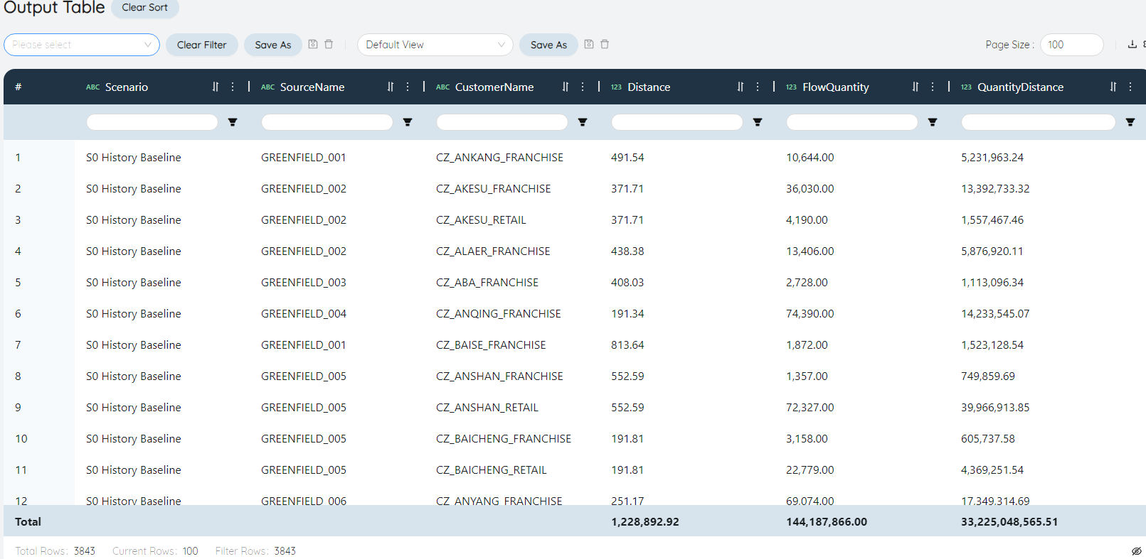
- OutputGreenFieldFlow
Shows the predicted FlowUnits, ServiceDistance sent to the client segment.
# How to predict optimization results? Build the Scenario.
In order to predict the optimization details of the site selection scheme, you can add site selection Sites to the Sites table, and run network optimization on the basis of the new Sites to get the optimization results.
# Model input
- Sites
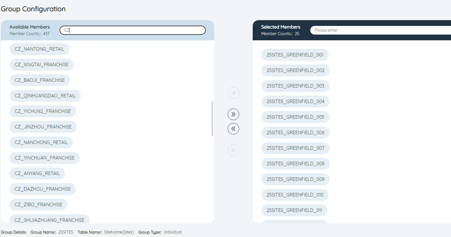
On the Sites summary interface, click the Add to Sites table button at the top, and select Replace current filter criteria to filter Value.
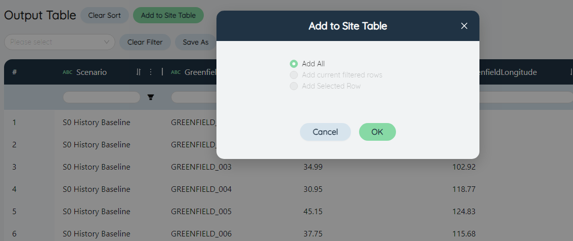
Go back to the Sites table and find that new Sites have been added.
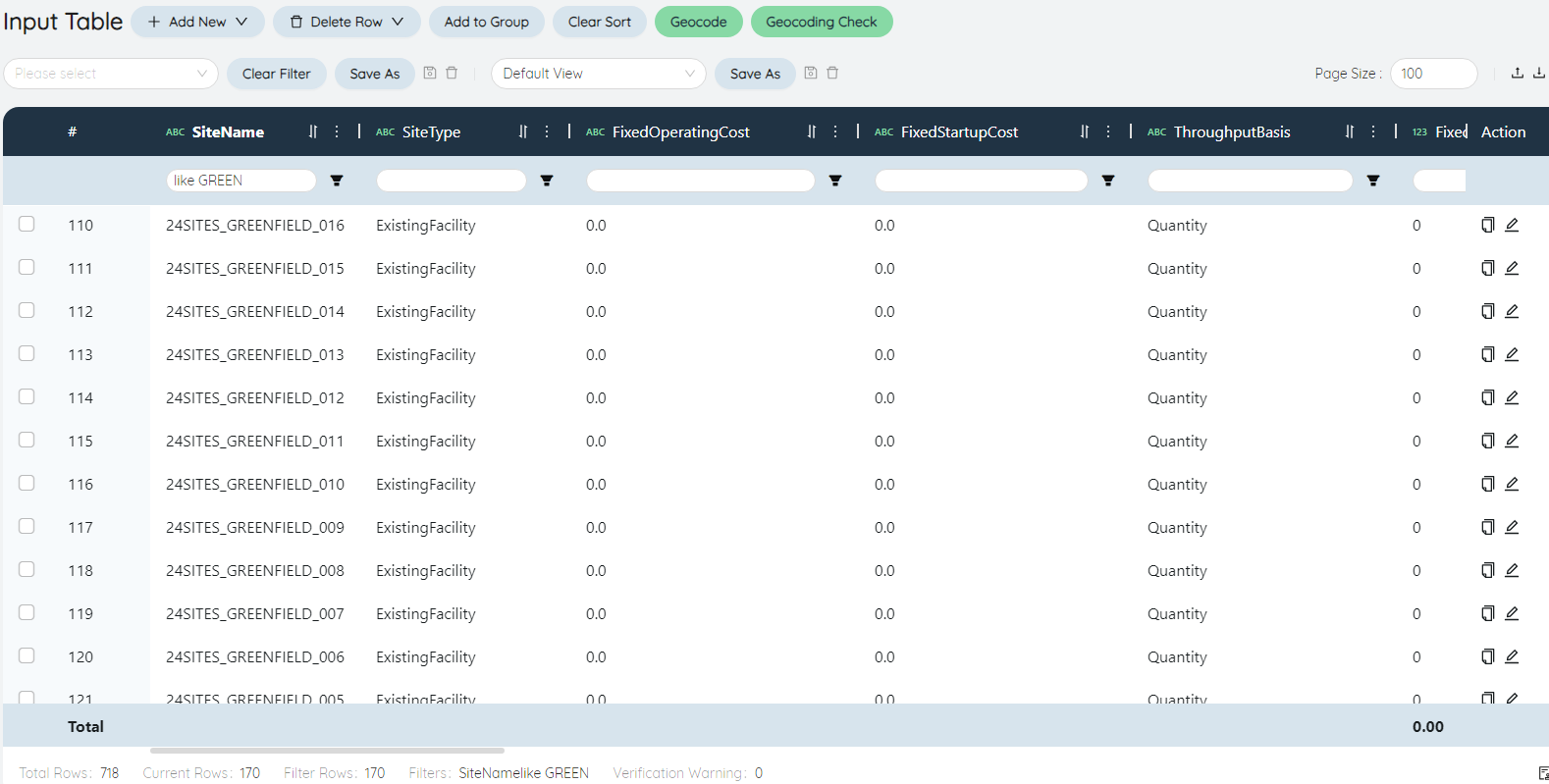
Create Groups for the 25 new sites, named 25SITES, and Type as Individual.
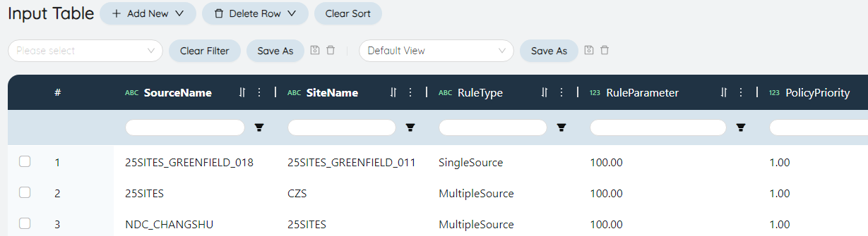
- SourcingPolicies
on the OutputGreenFieldFlow interface, delete all columns except the starting point Name and Customer Name in Excel, rename the Customer Name to Sites Name, add a Products Name column, and fill in the Value "down jacket".
Click Import on the SourcingPolicies interface, select Add as the import method, and add all the down jackets purchased from the new site to the customer's line to SourcingPolicies.
Add a line to purchase down jackets from NDC's main warehouse to Groups 25SITES.
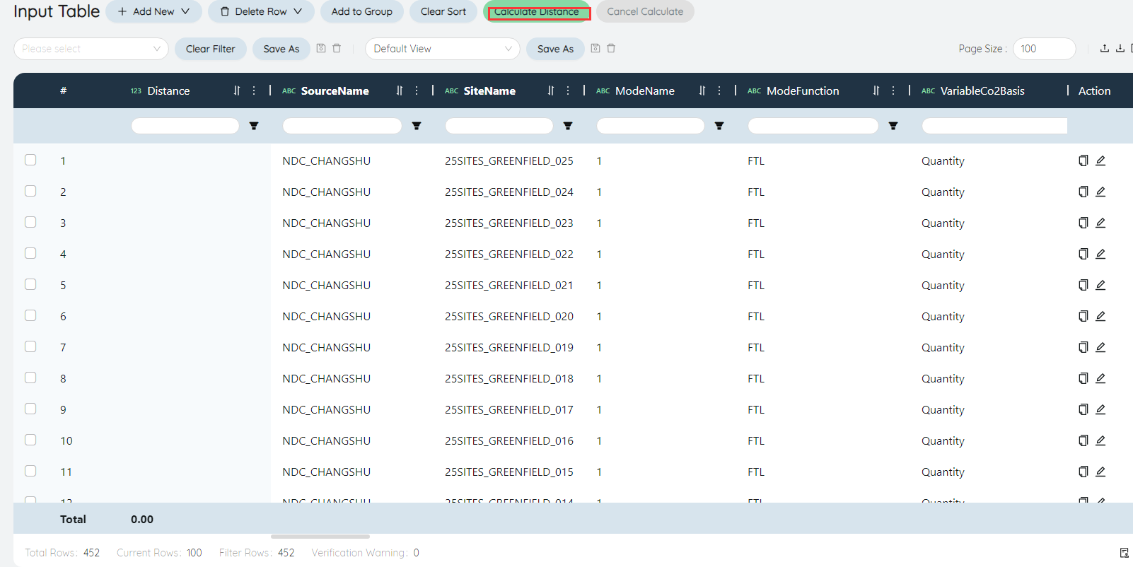
- TransportationPolicies
Click Export on the OutputGreenFieldFlow interface, delete all columns except the starting point Name and Customer Name in Excel, rename the Customer Name to Sites Name, add a Products Name column, fill in all the Value "Down Jacket", add a Transport ModeNameName column, Fill in all Value "2", add the Transport ModeName function column, fill in all Value "LTL", add VariableTransportationCost, VariableCostBasis, FixedShipmentCost three columns, fill in according to the TransportationCost of sub-warehouse-store.

Add ShipmentLane from NDC to each new location in the TransportationPolicies table. If the location City is the same as the original, TransportationCost also takes the original Value. If the location City is different from the original, TransportationCost takes the predicted Value of the total warehouse - sub-silo ( As shown below).
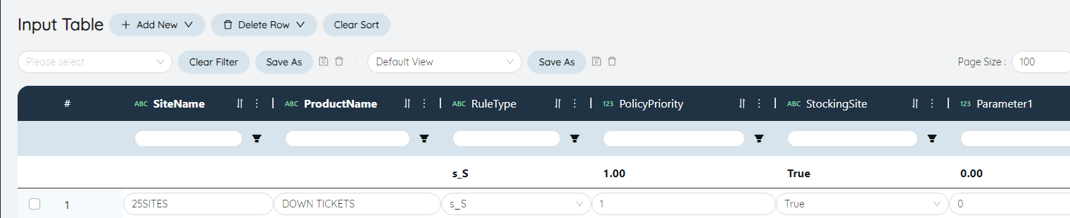
- InventoryPolicies
Add a new Sites policy to store down jackets.
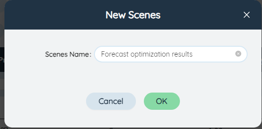
- Scenario
In the left function bar, select Scenario, click New Scenario, enter the Scenario name as prompted, and click Submit.

Create a new Scenario item C1
In the left function bar, select the Scenario item, click New Scenario Item, enter the Scenario item name as prompted, and click Submit.
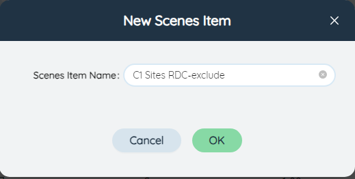

Edit Scenario Item C1
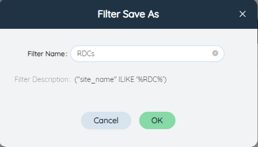
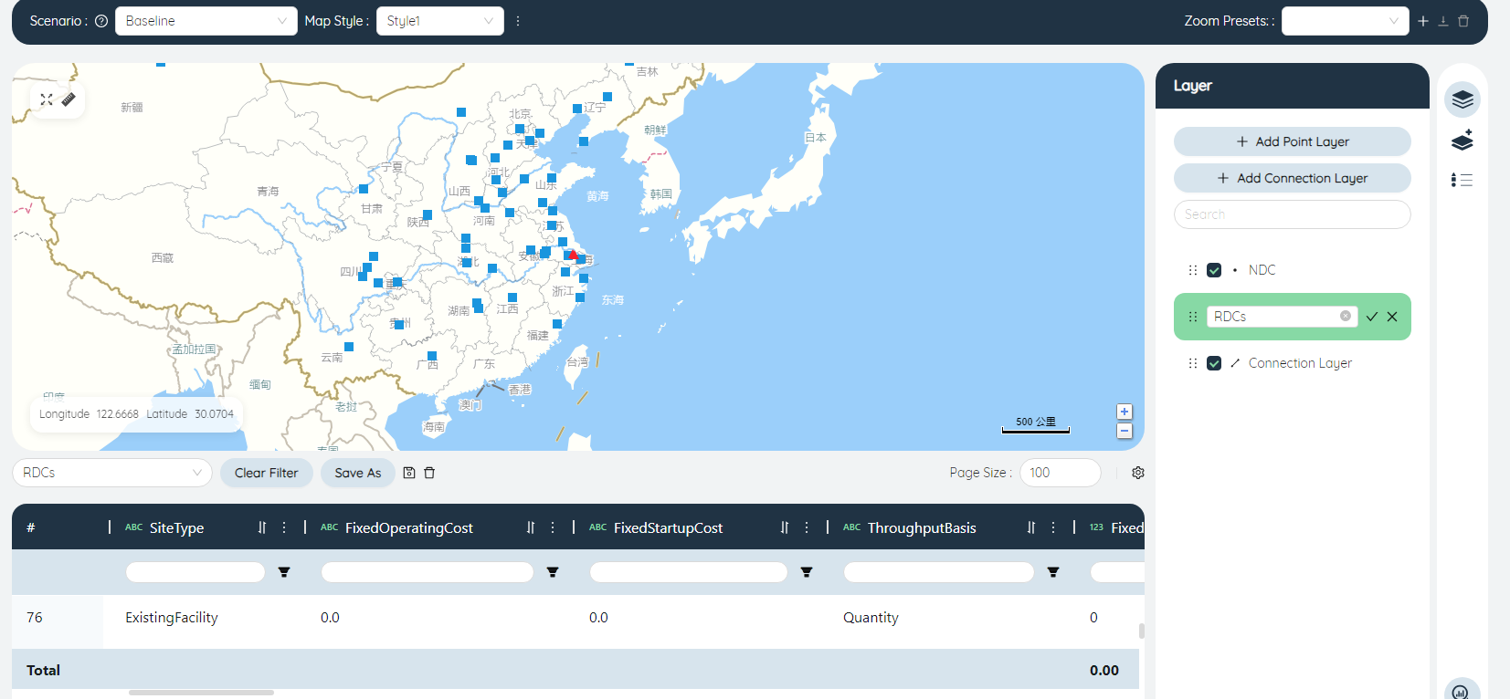
Select Sites in the association table, and the Sites Name is filtered according to the filter condition: "like RDC"
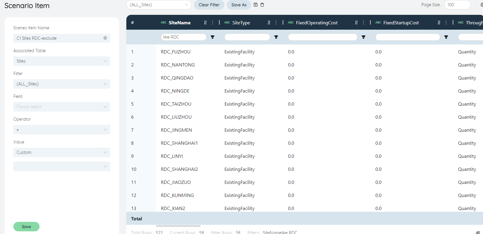
Click Save As Filter, name it RDCs,
Select RDCs for the filter, Status for the field, "=" for the operator, and "Exclude" for the Value.
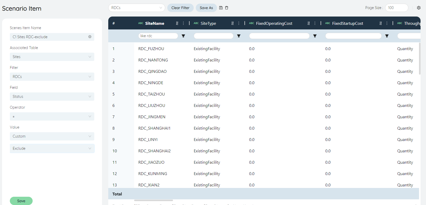
Click Save to see the Save Successful popup.
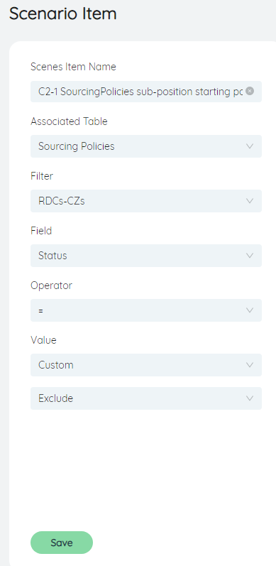
Create a new Scenario item C2-1
Named "C2-1 SourcingPolicies sub-position starting point exclude". The purpose is to have the model not take into account the lines from the original RDC.
Edit Scenario item C2-1
Fill in the prompts as shown in the figure below, and the filter condition is the starting point Name "like RDC".
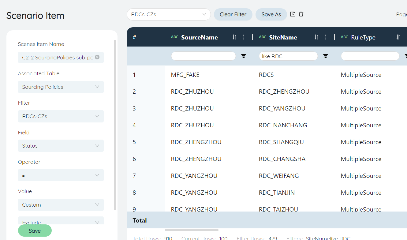
Create a new Scenario item C2-2
Named "C2-2 SourcingPolicies sub-position exclude". The purpose is to have the model not consider lines that end in the original RDC.
Edit Scenario item C2-2
Similar to C2-1, the filter condition is Sites Name "like RDC".
Create a new Scenario item C3-1
Named as "C3-1 TransportationPolicies sub-position starting point exclude". The purpose is to make the model not consider the lines starting from the original RDC.
Edit Scenario Item C3-1
Similar to C2-1, the filter condition is the starting point Name "like RDC".

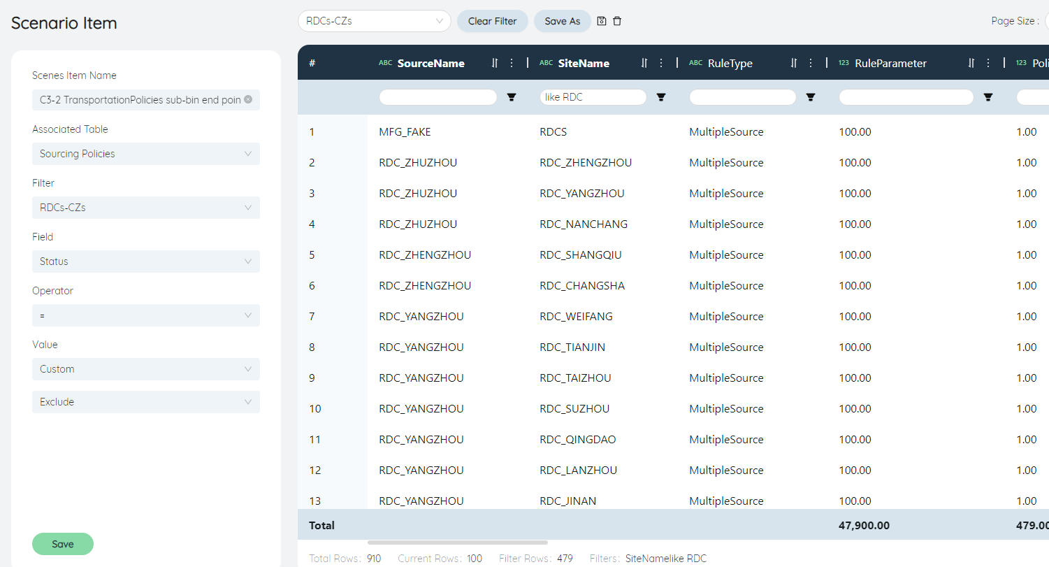
Create a new Scenario item C3-2
Named "C3-2 TransportationPolicies sub-bin end point exclude". The purpose is to have the model not consider lines that end in the original RDC.
Edit Scenario item C3-2
Similar to C2-1, the filter condition is Endpoint Name "like RDC".
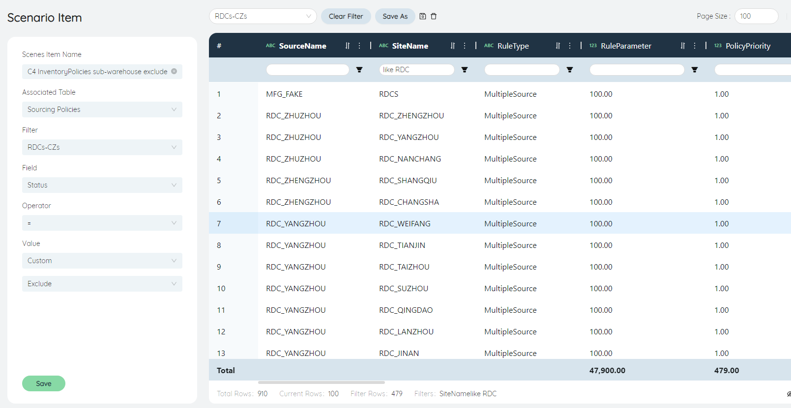
Create a new Scenario item C4
Named "C4 InventoryPolicies sub-warehouse exclude".
Edit Scenario Item C4
Fill in the prompts as shown in the figure below, and the filter condition is the SiteName "like RDC".
Edit the Scenario "Prediction Optimization Results" as shown below.
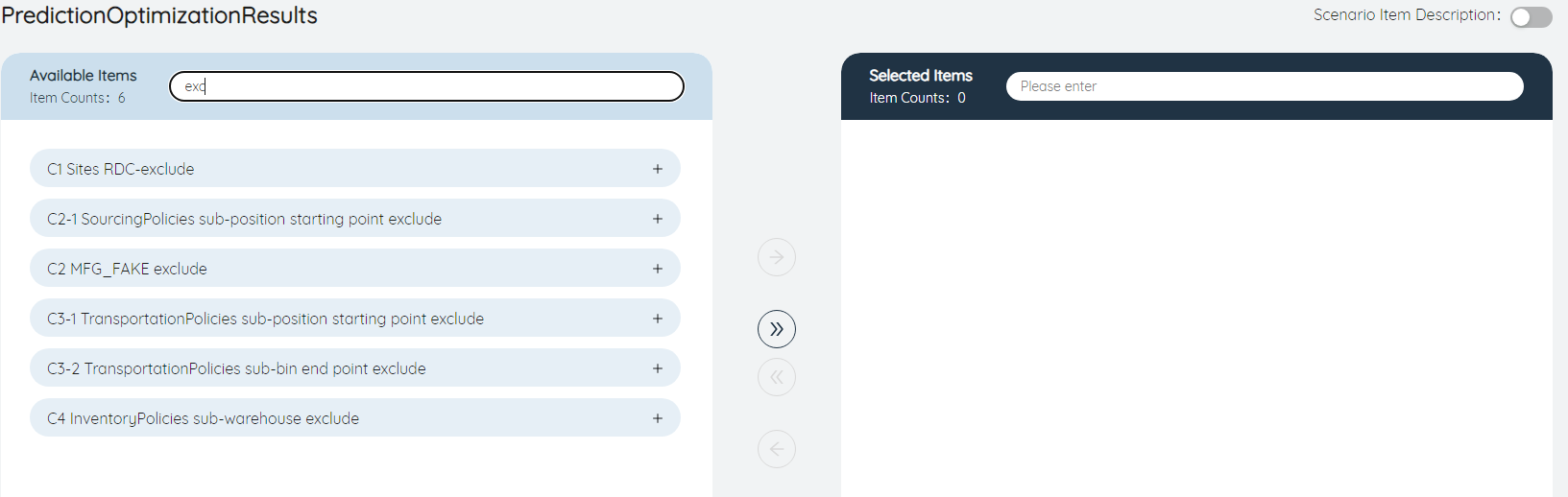
# Model output
Run Scenario: Predict optimization results on the online task list.
Export output table: Flow Details. Analyze optimization results outside the model.
# Scenario analysis and comparison
Do data analysis on the Flow Details table exported from SCATLAS.
Generally, it includes the following three aspects: warehouse network layout comparison, cost composition comparison, and ServiceLevel comparison.
There may be key metrics such as various shipping tiers, Country/Region/Warehouse, Traffic to Products, TransportationCost, ServiceDistance, ServiceHour, etc.
# Warehouse network layout comparison
Use the map tool that comes with SCATLAS to draw the warehouse network layout map of the Baseline and the optimized model.
- Draw Baseline's warehouse network layout map:
Click the map on the left function bar, click the New Map button, and fill in "Baseline" for the Map Name.
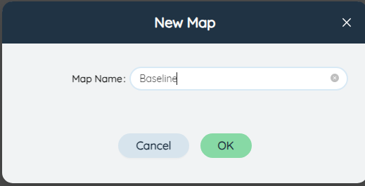
Click Submit. Enter the map editing interface.
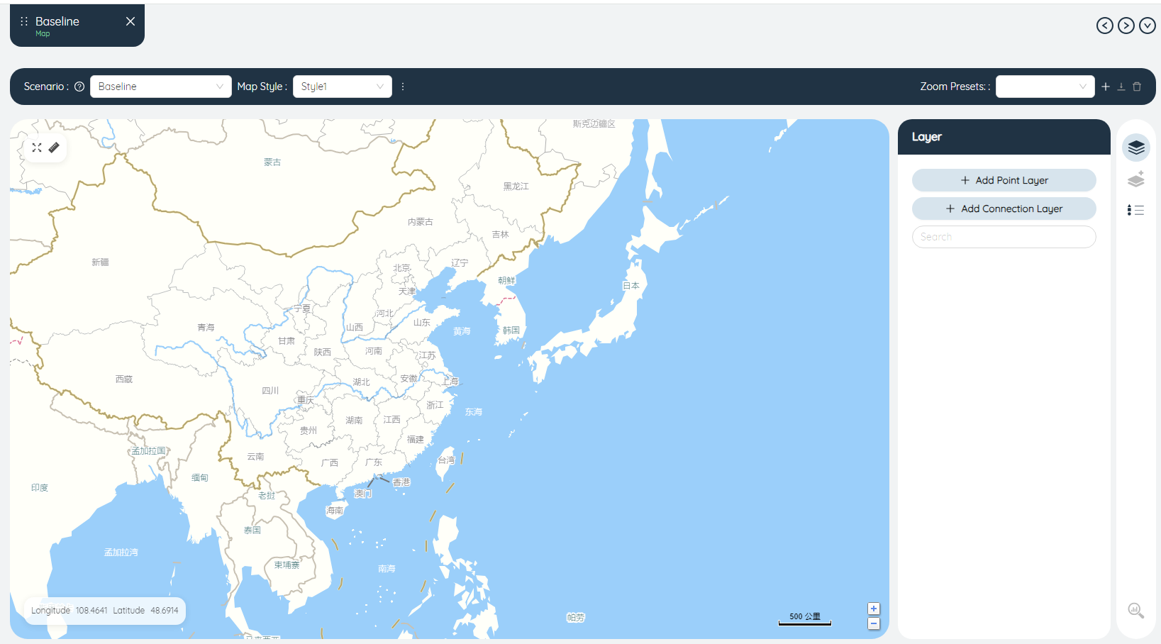
First add Sites information on the map, click the "Add Point Layer" button, and click the "Display Data" button.
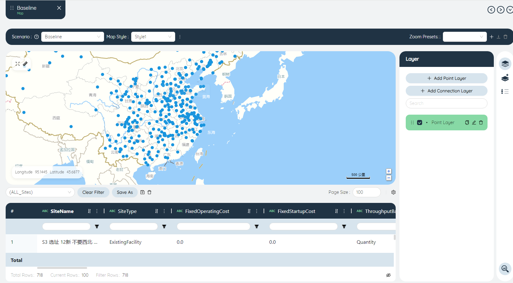
Add a point layer:
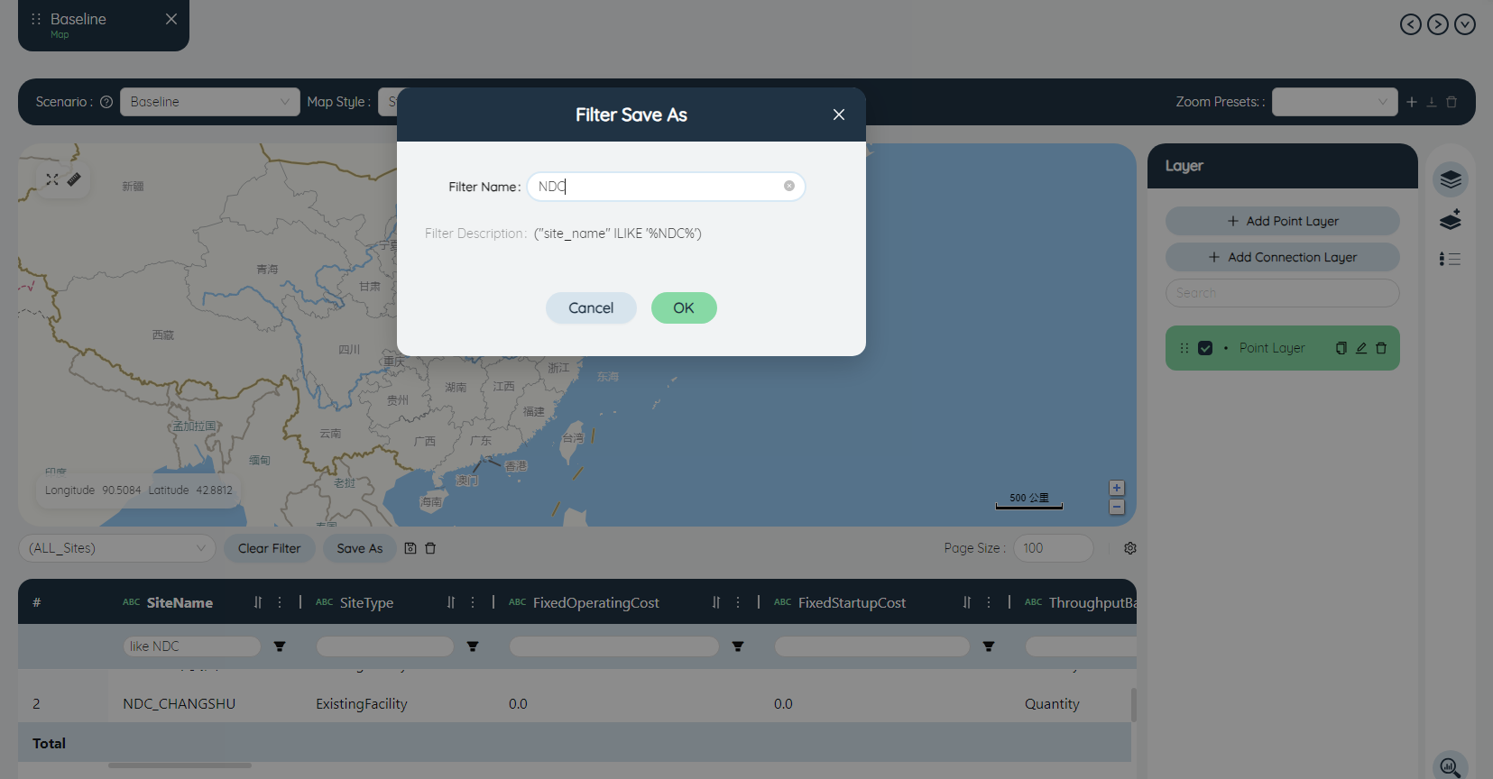
Enter NDC in the filter box, click Save Filter As, name it "NDC", and click Submit.
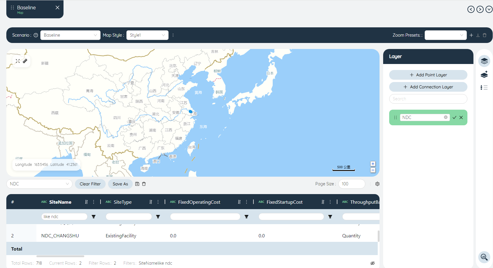
Filter to select NDC, rename the point layer to NDC, and click √.
In the layer editor, choose Triangle for Shape, fill in 15 for Size, and choose Red for Color.
You can see that a small red triangle appears at the location of the Changshu General Warehouse on the map.
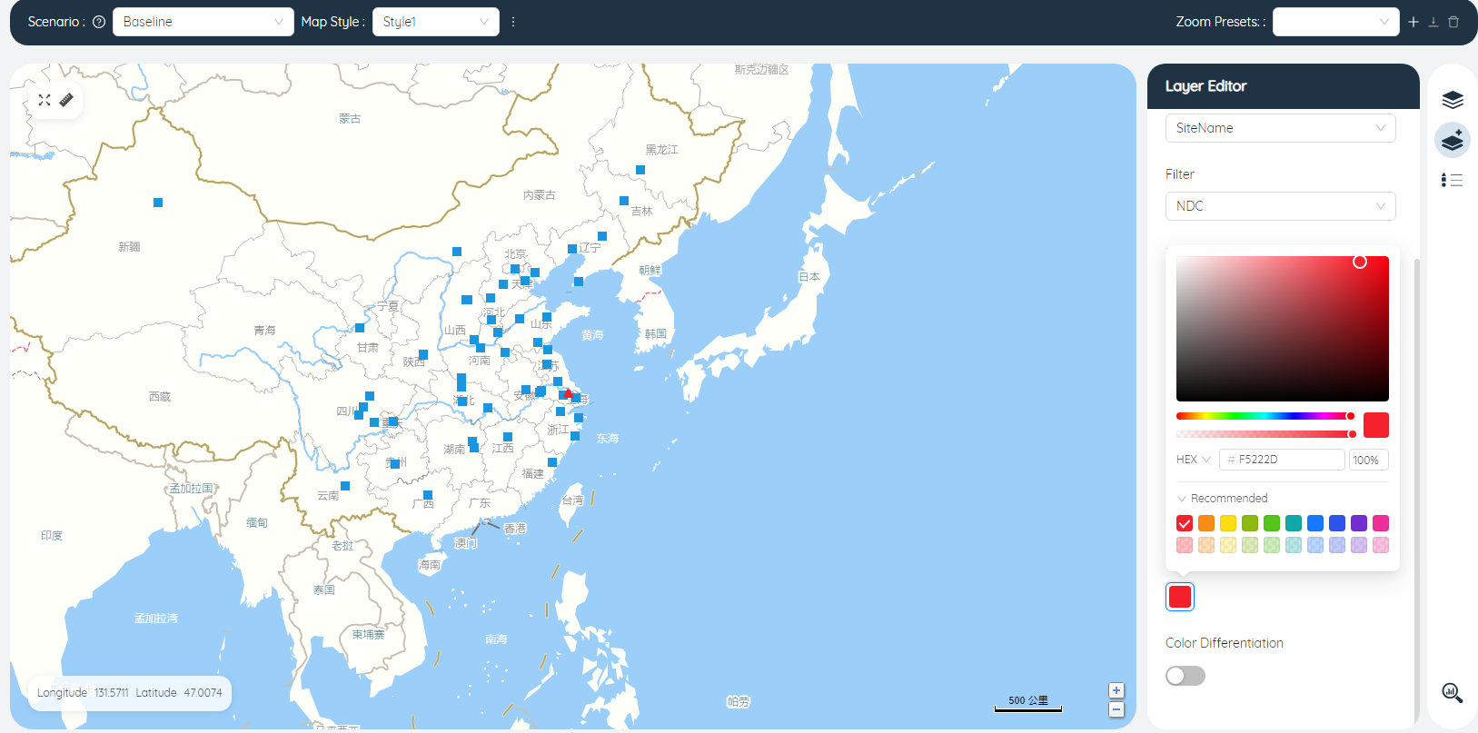
Follow the prompts in the image below to add a point layer in the same way: RDCs, marked with small blue squares.
Add a line layer:
Select Baseline for Scenario, select NDC for Start Name, RDC for Sites Name, and save as the filter "NDC-RDC".
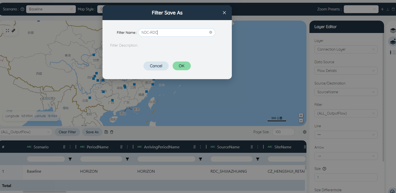
Choose red for the color, rename the line layer to NDC-RDC, and click √.
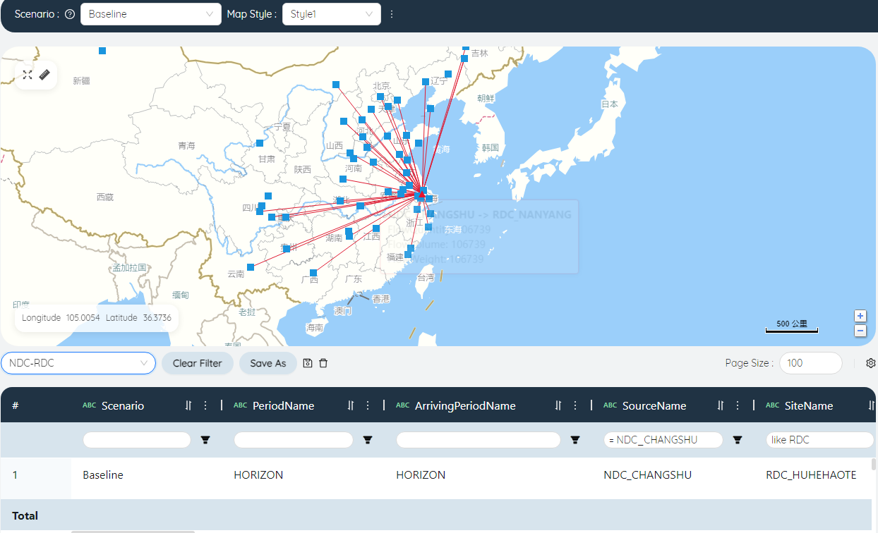
Follow the prompts in the image below to create a new layer "RDC-CZ" in the same way.
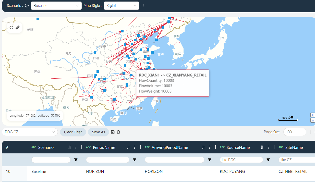
Baseline's warehouse network layout is completed.
- Draw the optimized warehouse network layout map
Create a new map and name it "Optimized Warehouse Network Layout".
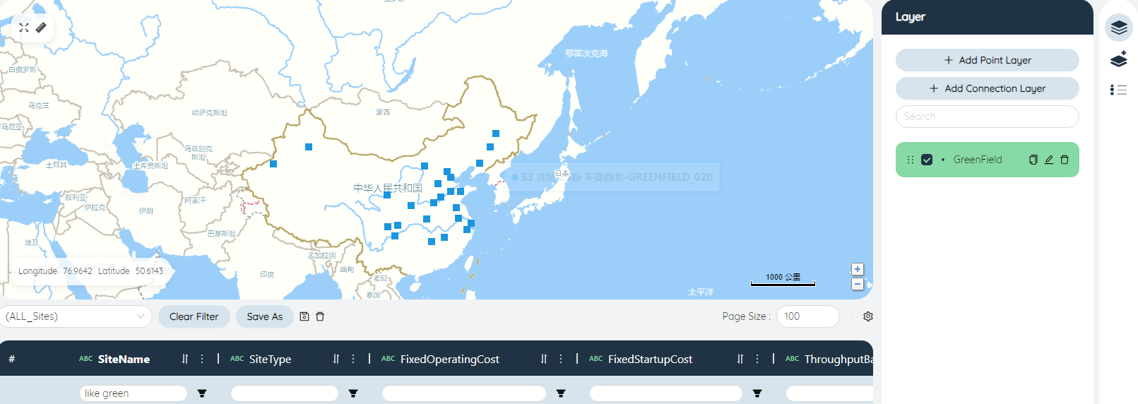
Add a point layer:
Scenario selects "Prediction and Optimization Results", clicks Add Point Layer, and creates a new Sites layer as prompted as shown below.
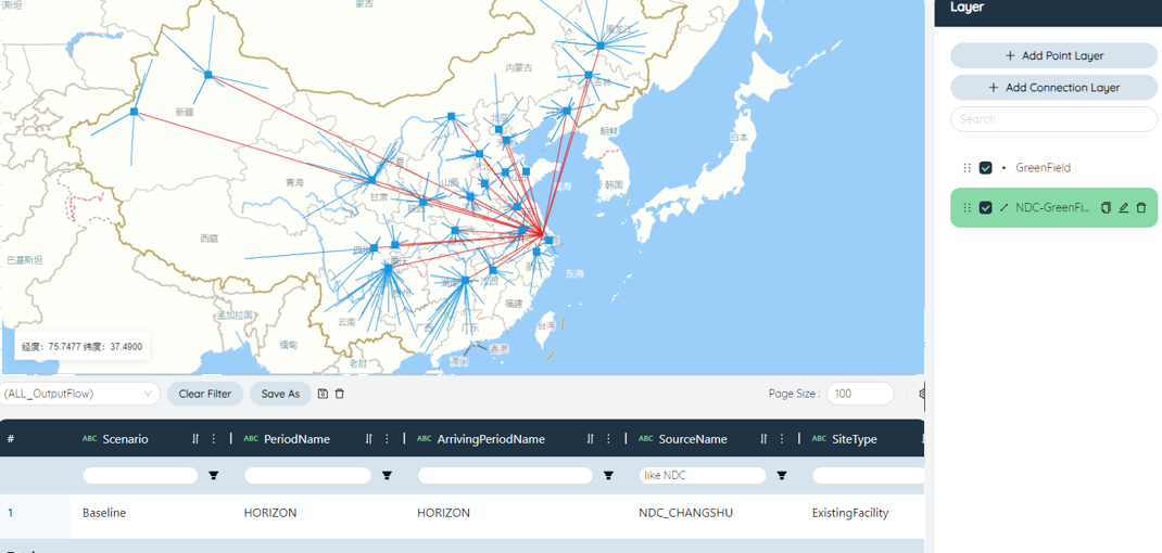
Add a line layer:
Filter out the lines from the NDC to the new Sites in the Flow Details table, and create a line layer as prompted as shown below.
Filter out the line from the new site to the store in the Flow Details table, and create a line layer as prompted as shown below.
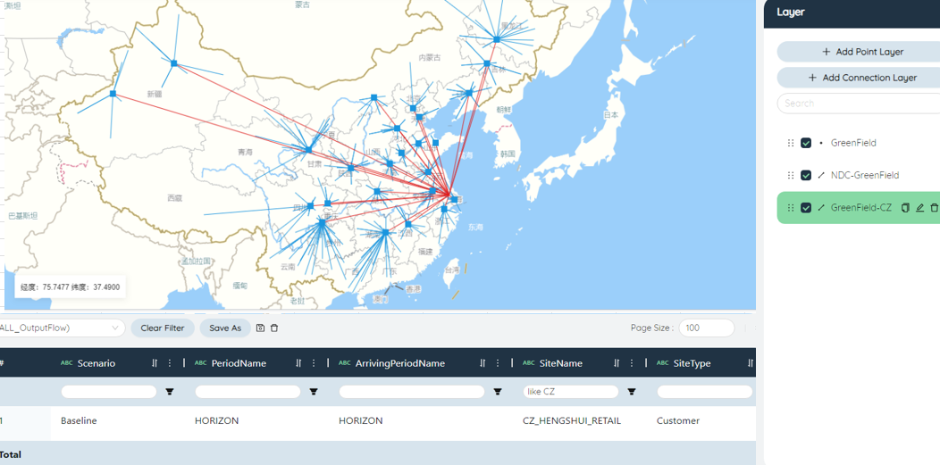
After optimization, the layout map of the warehouse network is drawn.
- Comparison of warehouse network layout before and after optimization:
Baseline's warehouse network layout (58DC)
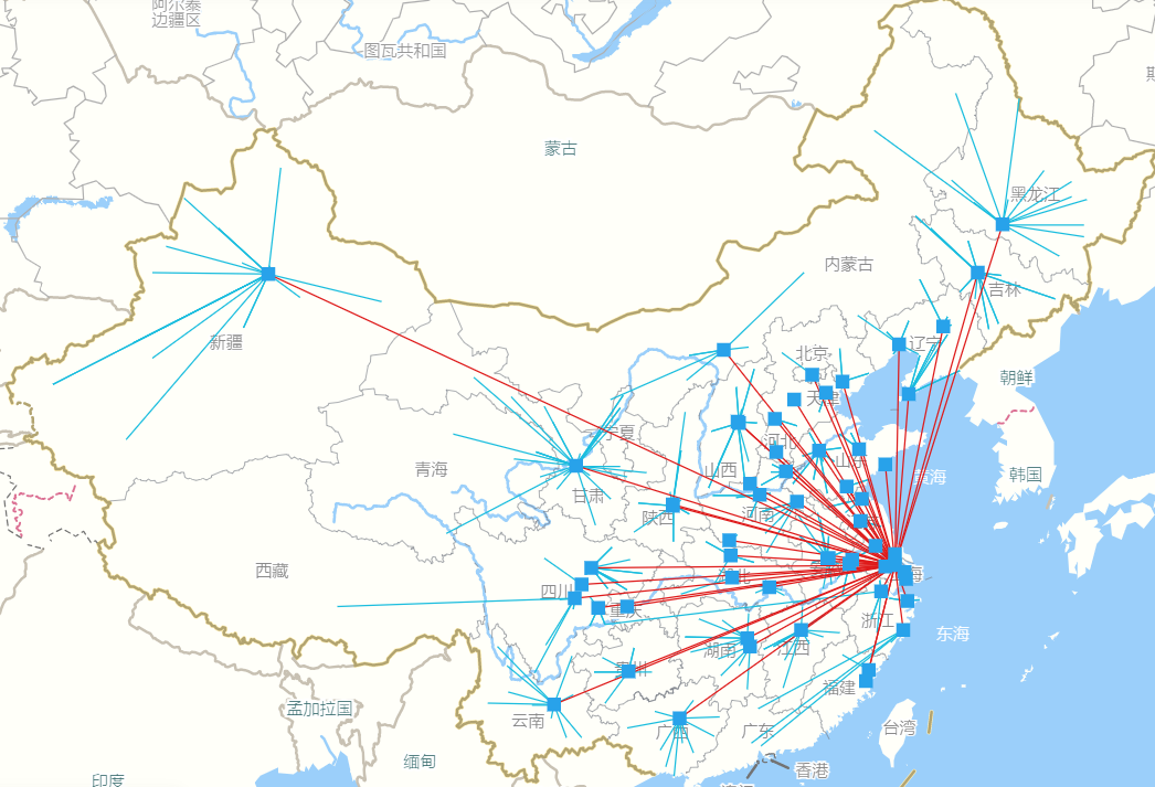
Optimized warehouse network layout (25DC)
After optimization, the warehouse Quantity is reduced by 33.
Among the 25 warehouses in the optimized plan, there are  18 original warehouses and
  7 new warehouses.
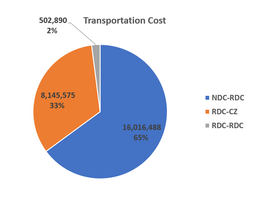
# Cost comparison
After optimization, TotalCost decreased by 3.24%, about 987,000 yuan.
Among them, the TransportationCost of the NDC-RDC (total warehouse-sub-warehouse) segment decreased by 4.99% to about 1.115 million yuan; the TransportationCost of the RDC-CZ (sub-warehouse-store) segment increased by 1.54% to about 125,000 yuan.
# ServiceLevel comparison
The ServiceLevel of the Northwest and Southwest regions of Baseline does not meet the 98% requirement line.
After optimization, the service satisfaction rates in all regions have reached the requirements.
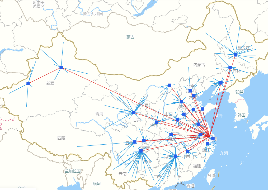
# Mock Case 2 LX Milk
# How to reflect the historical situation? Build the Baseline benchmark model.
# Project scope
Production and sales plan SnapshotDate range: June 2017
Facility overview: 14 milk sources, 16 factories, 55 customers
Products: 1 raw material (raw milk, ShelfLife 9 days), 20 finished products (SKU), 16 long-term products, 4 short-term products (ShelfLife 15 days)
TotalDemand: 78,484 tons
Mode of transportation: truck, rail, ocean
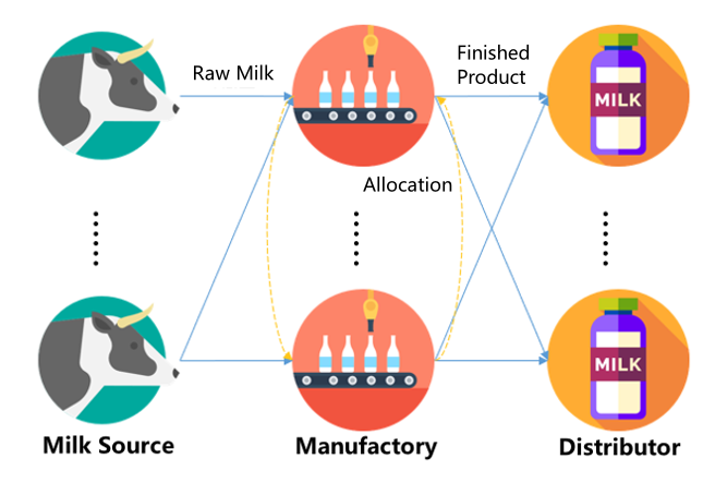
Products Flow Type:
Raw milk distribution: milk source - factory
Finished Product Distribution: Factory - Customer
Allocation: Allocation of raw milk and finished products between milk sources and factories
# Raw Data Download
# Model input
User notice:
Before running the model, the data is entered in tabular form.
The model input required by different algorithms is different, which is divided into required input and optional input. For example, the required input table of NO is Periods, Products, Sites, CustomerOrders, ProductionPolicies, SourcingPolicies, TransportationPolicies, InventoryPolicies. S&OP (Rolling Production Planning) involves more, including input tables such as WorkCenters, ProductionProcess, and BOM (BOM) required to describe the production side.
Next, the input table required by the Baseline benchmark model will be introduced, including the meaning of the fields used, the corresponding relationship between the value of the field and the original data.
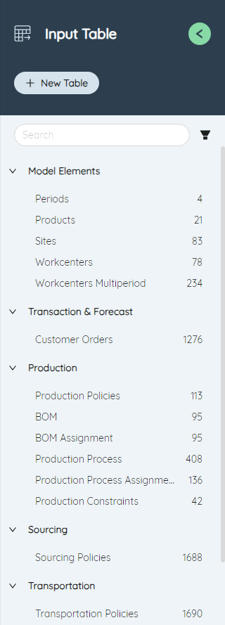
- Periods
According to the scope of the project, starting from early June 1, 2017 to the end of late July 1, it is divided into 3 Periods: the first, middle and last days.
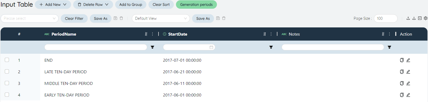
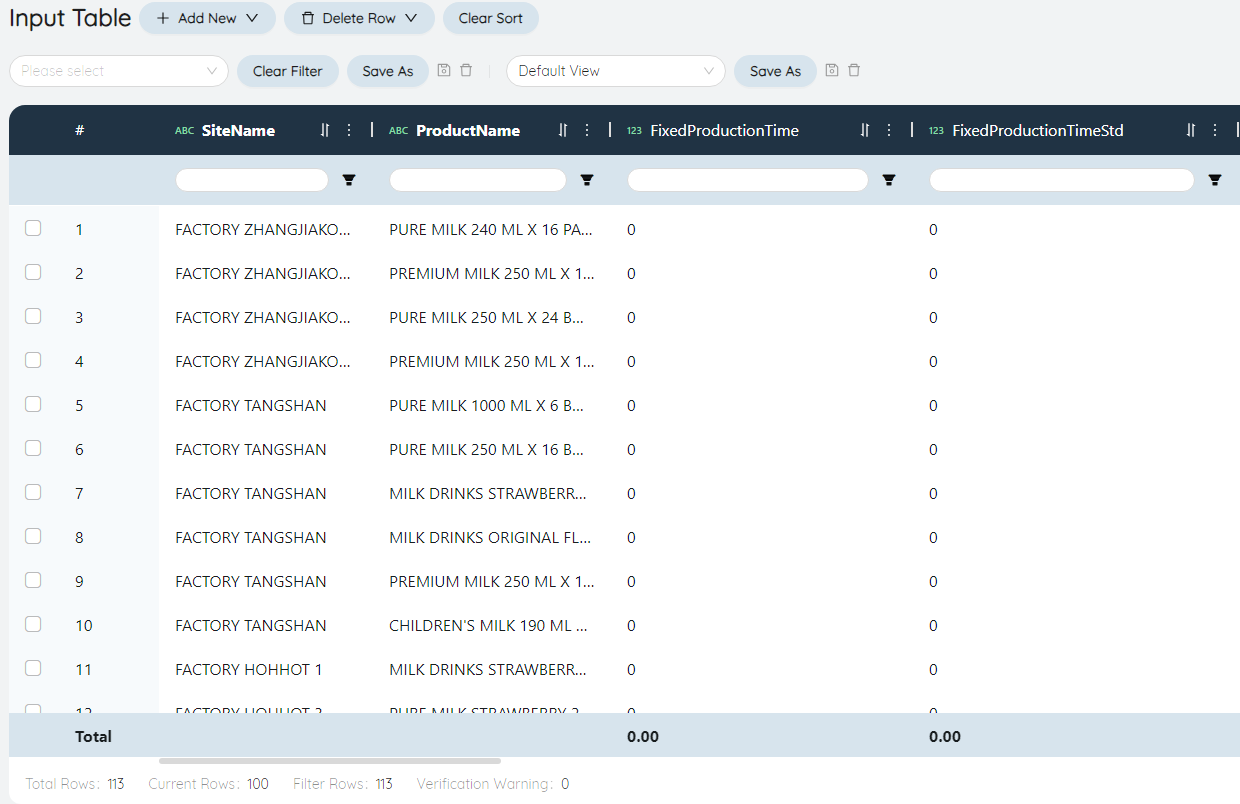
- Products
Contains information such as Products Name, Price, ShelfLife, Products category, Products category (ShelfLife length).
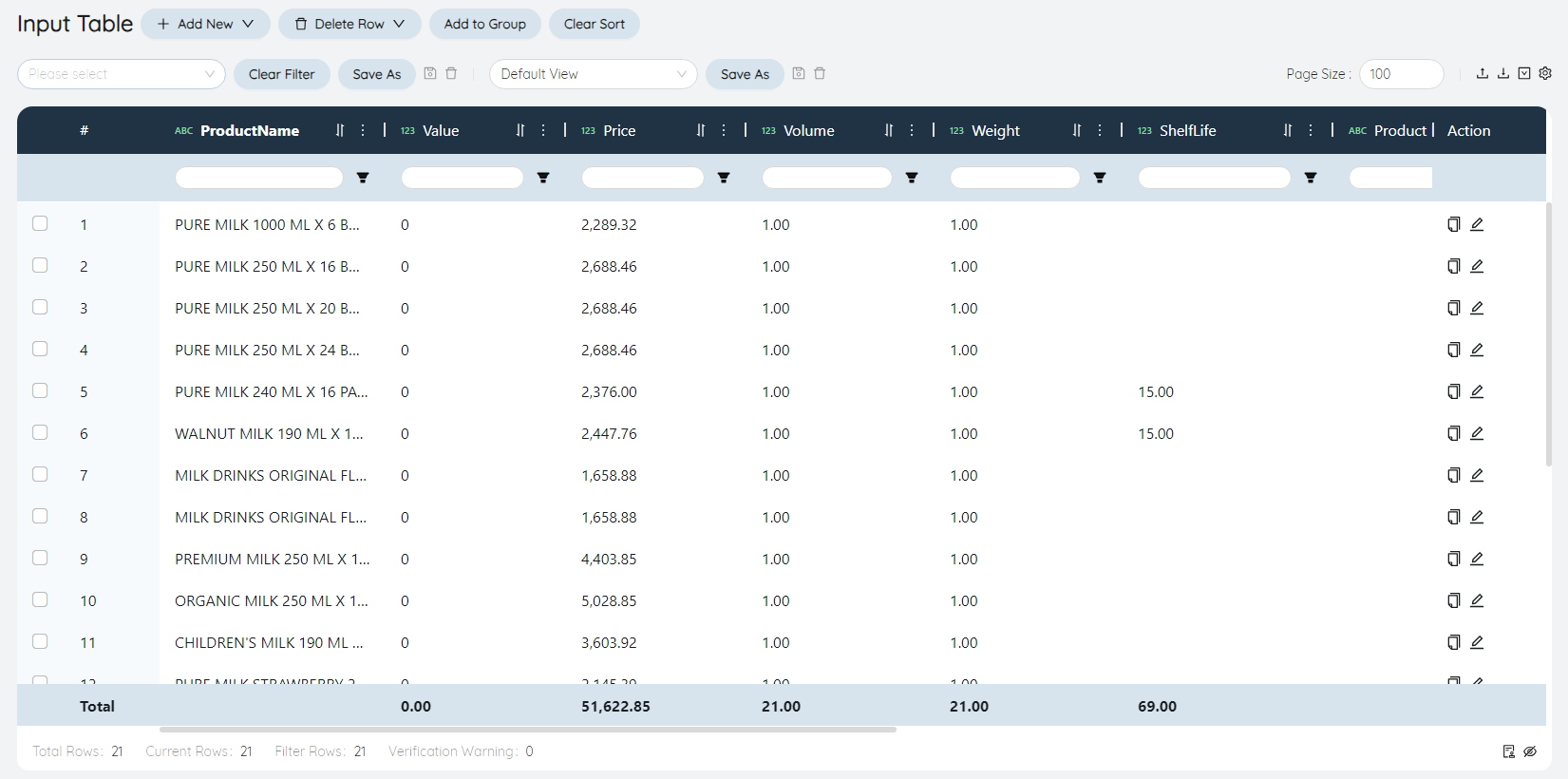
Products Name
Raw milk 1 raw material + 20 finished products, a total of 21 lines of data.
Price
Fill in according to the field of **Products ex-factory price (yuan/ton)** in the original data - Products data .
ShelfLife
Raw milk ShelfLife is 9 days, short-term products ShelfLife is 15 days, and long-term products ShelfLife is not considered.
Notes
Fill in according to the Products category in the original data - Products data (optional).
Custom21
Fill in (optional) based on the Products category in the raw data - Products data .
- Sites
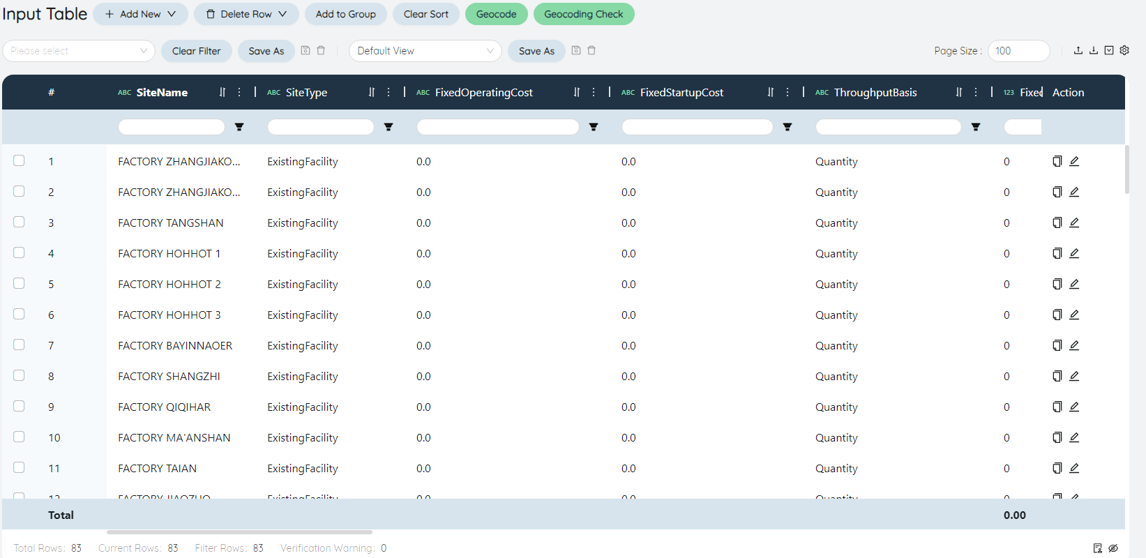
Sites Name
1 Dummy fake factory (used for production and transportation of InitialInventory) + 14 milk sources + 16 factories + 52 Province office/large dealer customers, a total of 83 pieces of data.
Sites Type
The fake factory, milk source and factory are ExistingFacility, and the customer is Customer.
City, Province share
Fill in the corresponding Province city information according to the original data - customer location , factory location , and milk supply location .
Latitude/Longitude
After filling in the Province city information in the Sites table, click Geocode to get it automatically. If there is longitude and latitude in the raw data, it is unnecessary to do so.
Sites family
Milk source, factory, Province office customers, large dealer customers.
- WorkCenters
WorkCenters generally refer to production lines or workshops, including FixedOperatingCost (which can be set as a ladder), ConstraintValue benchmarks, and other information.
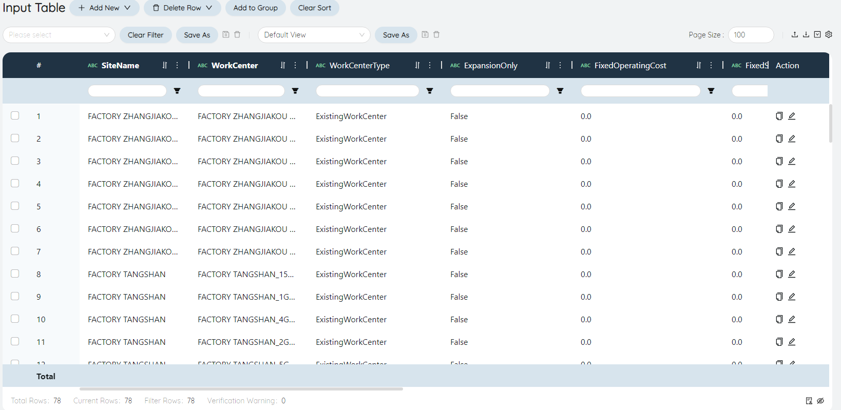
**WorkCenters**
Factory Name and Equipment Groups Name fields of the capacity table in the original data. The naming rule is <Factory Name>_<Equipment Groups Name>
Sites Name
Fill in the factory corresponding to WorkCenters
ConstraintValue benchmark
It is used to specify the unit benchmark of ConstraintValue in ProductionProcess. Each WorkCenters in this Scenario is Hour, and production is limited by SnapshotDate.
- WorkCenters Multiple Periods
You can set the FixedOperatingCost, on/off cost, Co2 and other information of each WorkCenters in Periods here.
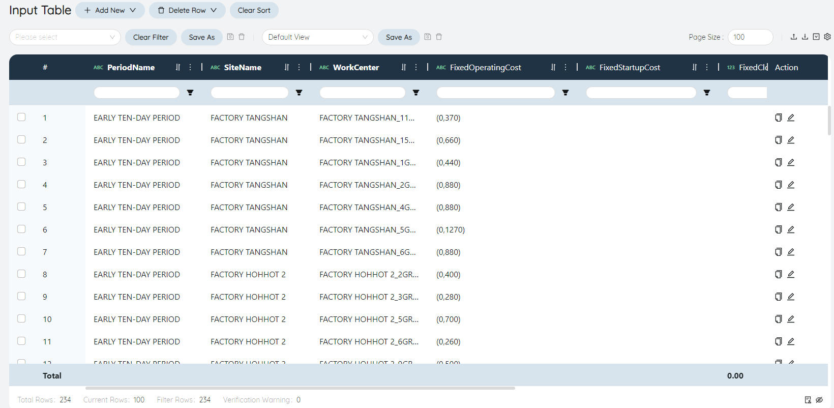
Periods Name
Early/mid/late
FixedOperatingCost
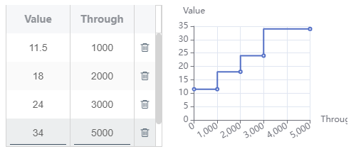
general filling format is: (OperatingCost of the first step, upper limit of ThroughputLevel of the first step), (OperatingCost of the second step, upper limit of ThroughputLevel of the second step). In this Scenario, the ThroughputLevel upper limit is used to set the capacity upper limit of each Device Groups per Periods.
capacity in the original data is the upper limit of the ThroughputLevel of each WorkCenters, which is filled in ( 0 , here).
- CustomerOrders
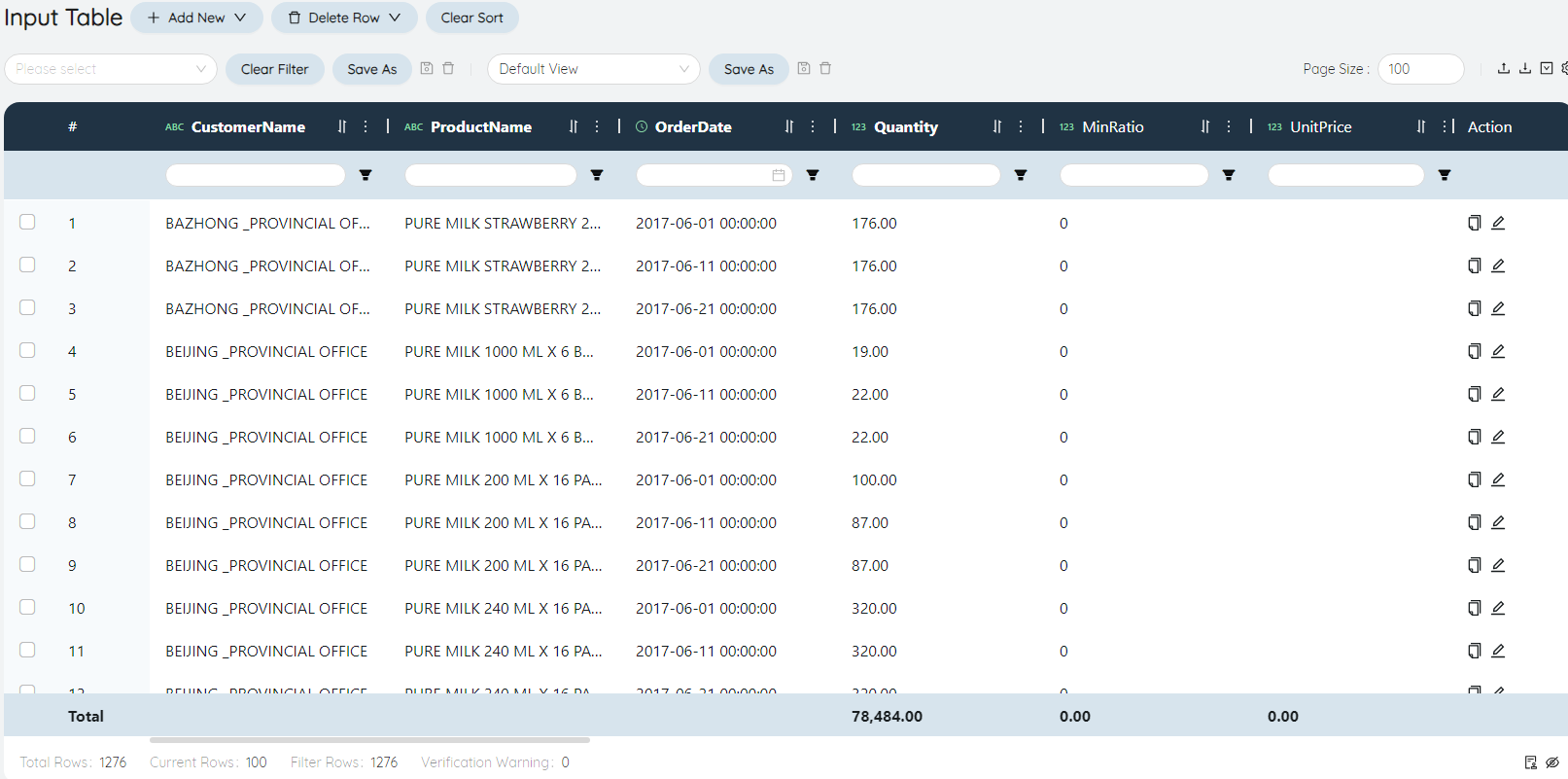
Based on raw data - customer needs .
OrderDate
Fill in the first day of each Periods in the first, middle and last days, for example: the first day is 2017/6/1.
- ProductionPolicies
The milk source produces raw milk, the factory produces finished products, and the Dummy fake factory produces finished products (short-term/long-term products).
- BOM
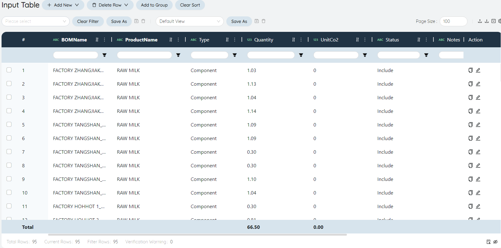
BOM Name
BOM (BOM for short) is a list of raw materials for a factory to produce a product, and the naming rule is <factory>_<finished product Name>_BOM.
Products Name
Fill in the raw material of the BOM. In this Scenario, the raw material of all Products is only raw milk.
Quantity
According to the original data - raw milk consumption per ton of finished product (tons)** in BOM raw milk consumption .
- BOM Assignment
This table exists to associate the BOMName with Periods, Sites (production), and Products.
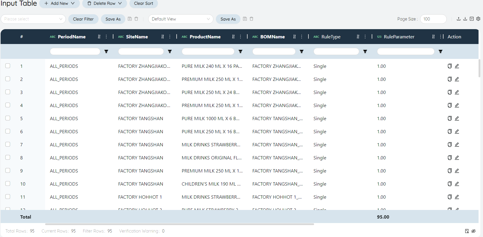
Periods Name
The BOM of the Products produced by each Periods factory is the same, no need to distinguish, fill in ALL_PERIODS.
BOM Name
BOM (BOM for short) is a list of raw materials for Products, and each factory produces the same Products with different BOM Names.
- ProductionProcess
ProductionProcess displays the relevant information of the process, one process per line, that is, the attributes of the process of each Periods and each WorkCenters producing each Product, including the work order of each process in the process, VariableProcessCost, UnitProcessHour and other information.
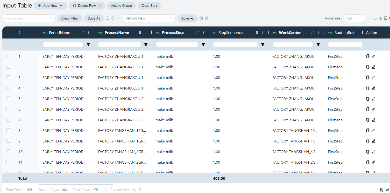
Periods Name
Early/mid/late.
ProcessName
Each equipment Groups produces the ProcessName of each Product, and the naming rule is <WorkCenters>_<Products Name>_PROCESS
Process Name, StepSequence
The process of each process has only one step: make milk, and the order is naturally 1.
**WorkCenters**
Fill in <WorkCenters> in ProcessName in order to associate the process with WorkCenters.
VariableProcessCost
From Raw Data - Production VariableCost . Different WorkCenters may have different ProductionCost for the same Product.
UnitProcessHour
process coefficient in the original data . The number of ProductionProcess hours required to complete the operation.
OrderLotSize
From raw data - production batches .
- Production Process Assignment

Associate ProcessName with Periods, Sites (production place), Products Name. The filling method is similar to BOM Assignment.
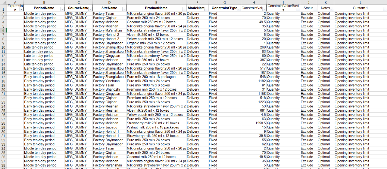
- ProductionConstraints
The ProductionConstraints of the Baseline model are actually the planned raw milk supply Quantity of each milk source in the first, middle, and later days, with a total of 14*3 (42) bars.
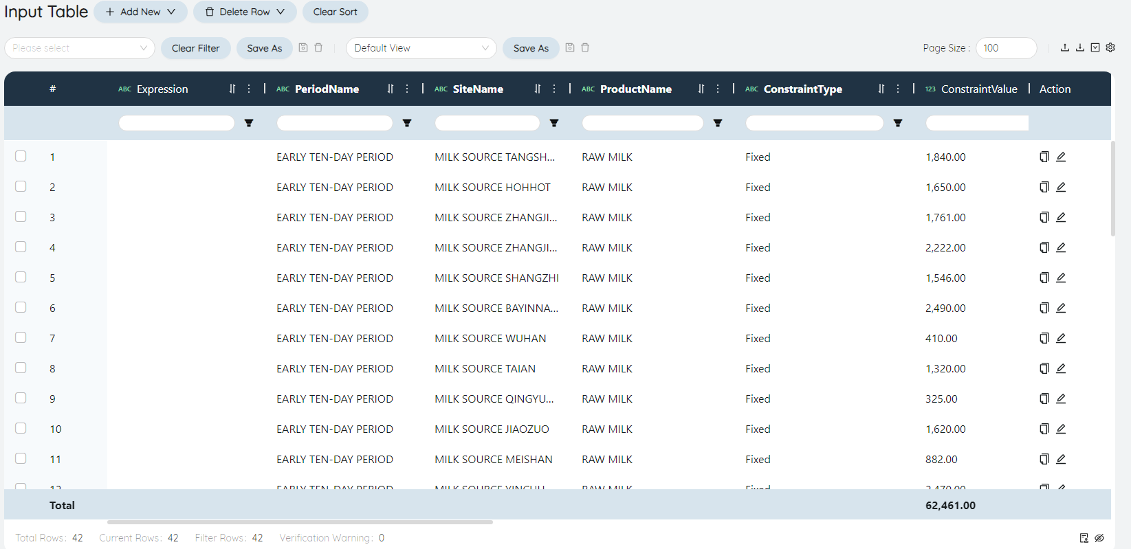
ConstraintType
Raw milk Quantity is essential, fill in Fixed.
ConstraintValue
From raw data - plan to have raw milk available .
- TransportationPolicies
Including Dummy's fake factory-factory, milk source-factory, transfer between factories, factory-customer's TransportationCost information of various modes of transportation ModeName. A total of 1690 pieces of data.
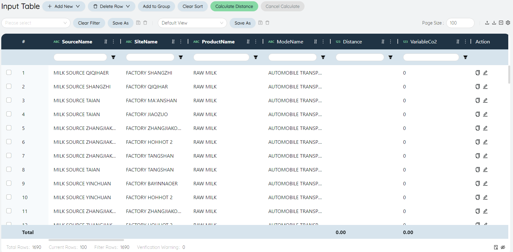
special data
The route that ships all Products from the fake factory MFG_DUMMY to the factory's individualGroups MFG is for the model to calculate the InitialInventory Quantity by itself, without affecting the analysis of the model results. The transportation ModeName is filled in at will, and the transmission is filled in the picture. VariableTransportationCost needs to be set much larger than other normal lines, so that the model chooses the Dummy fake factory when any other lines can't meet the needs. The model will automatically calculate the volume of goods sent by the fake factory to each factory, that is, InitialInventory. The following field filling instructions do not contain this special data.
Products Name, Shipping ModeNameName
According to the original data- manual distribution plan , the transportation route and transportation ModeName of each Product from the factory to the customer are obtained, and the transportation route and transportation ModeName of the raw milk from the milk source to the factory are obtained according to the raw milk allocation route and unit price . The raw milk is sent from the milk source to the factory, and the corresponding transportation ModeName is automobile transportation, with a total of 39 pieces of data; short-term insurance Products (4 kinds of finished products) are sent from the factory to customers, and the corresponding transportation ModeName is also automobile transportation, with a total of 553 pieces of data Data; Changbao Products (16 kinds of finished products) are sent from the factory to customers, and the corresponding transportation ModeName includes automobile transportation, sea transportation, and railway transportation, with a total of 1091 pieces of data; the transfer between factories only occurs in 1/2/3 of the factory Hohhot During the period, using trucks, Factory 2 transports raw milk to the outside, and receives 6 pieces of data for long-term warranty Products and short-term warranty Products from 1 and 3.
VariableTransportationCost, VariableCostBasis
VariableTransportationCost is filled in according to the original data - manual distribution plan , raw milk allocation line and unit price . In this scenario, the unit of Quantity is ton, and the VariableCostBasis corresponding to yuan/ton is Quantity.
- SourcingPolicies
Just fill in the Start, Sites, Products Name columns.
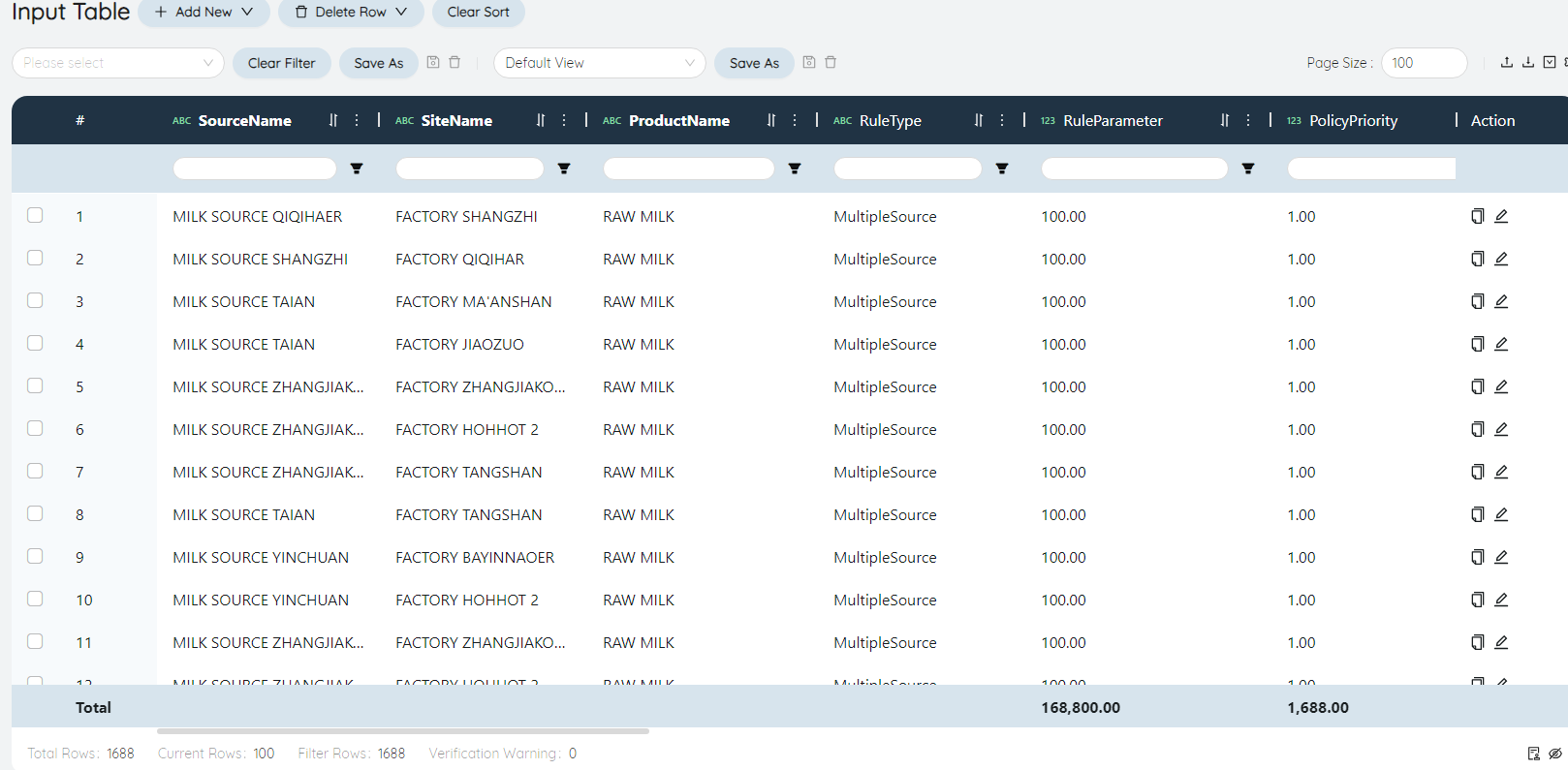
Similar to TransportationPolicies, you can directly copy the starting point, Sites, and Products Name columns of TransportationPolicies, with a total of 1690 entries. It is also possible to merge ShipmentLane between factories like in the picture.
- FlowConstraints
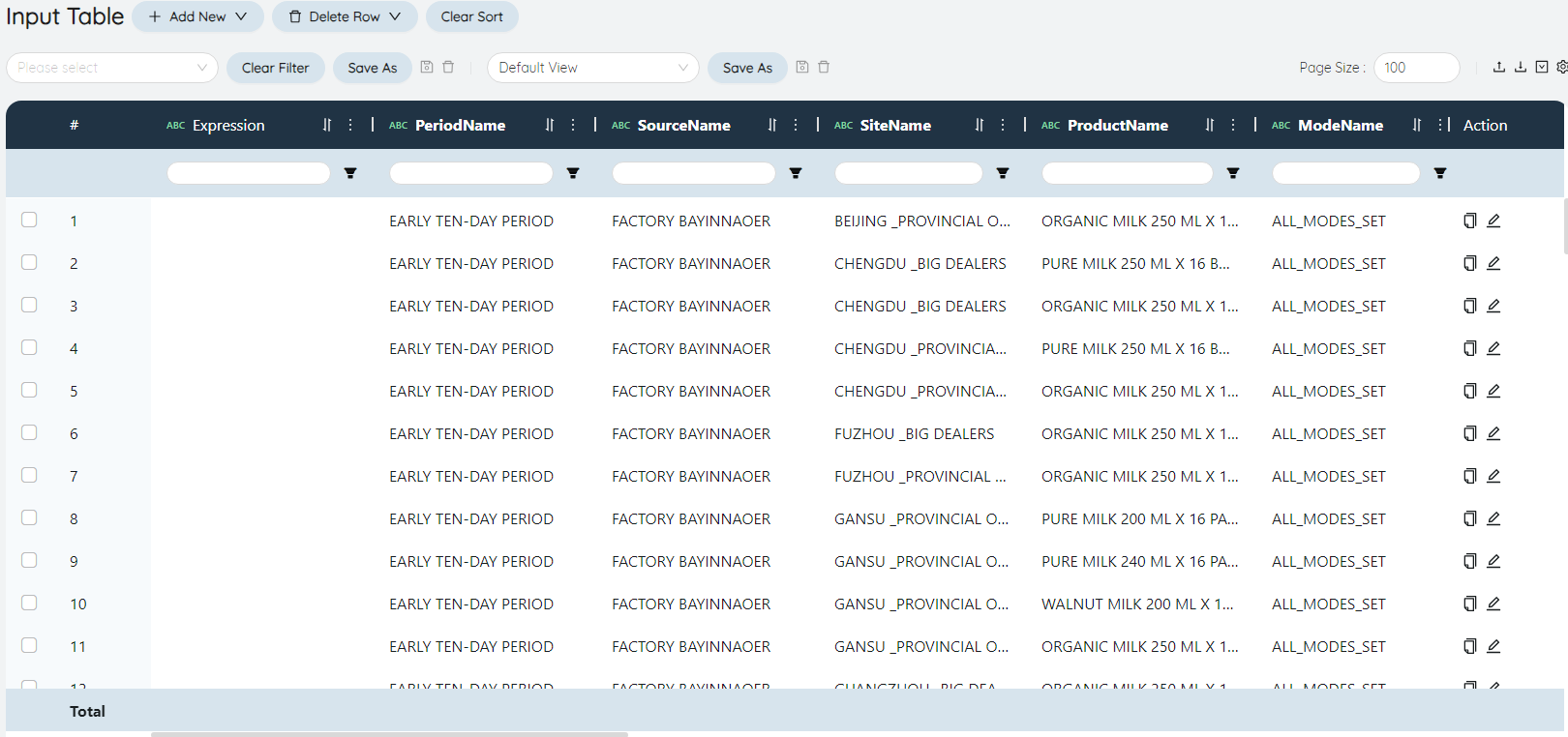
According to the original data - manual distribution plan to obtain the Quantity of each Product per Period and per route.
ConstraintType
Fill in Fixed.
- InventoryPolicies
The factory can store 20 kinds of finished products and 1 kind of raw material (raw milk).
Sites Name
Fill in the individualGroups of Sites: MFG.
# Model output
After filling in the input form, click the left function bar to enter the online task list, click Add task, check Baseline, select the algorithm "Network Optimization (NO)", click Add, and the model starts to run.
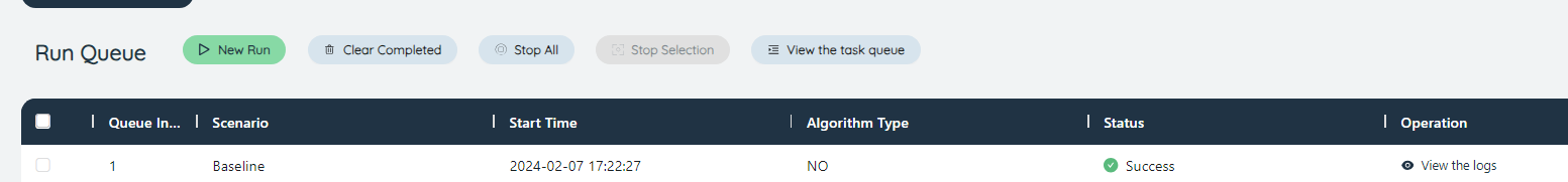
After the operation is successful, click the left function bar and select the corresponding output table to view.
- OutputNetworkSummary
Displays information such as Revenue, Profit, and segmented costs in the network.
Total Revenue
Calculated from the Price of Products in the model element.
Total Profit
Total Revenue-TotalCost
TotalCost
In this Scenario, it is equal to TotalProductionCost+TotalTransportationCost (in fact, TransportationCost includes the discard cost).
TotalProductionCost
In this Scenario, it is equal to the sum of Quantity*Unit Operation Cost of each Product produced by each WorkCenter.
TotalTransportationCost
In this Scenario, equals TransportationCost + drop cost.
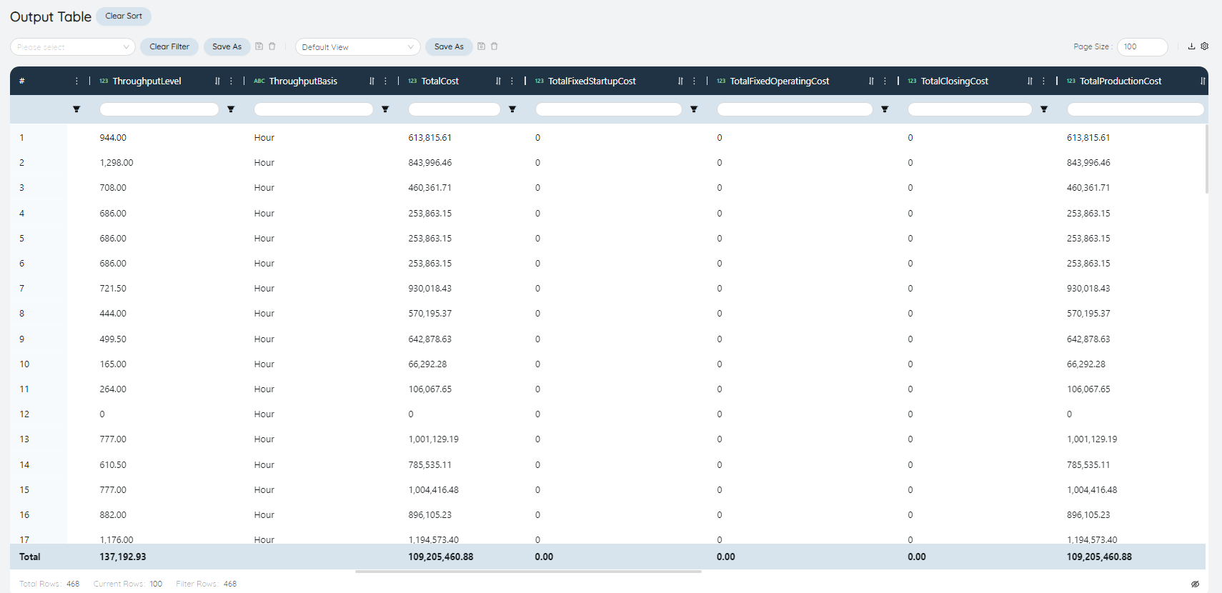
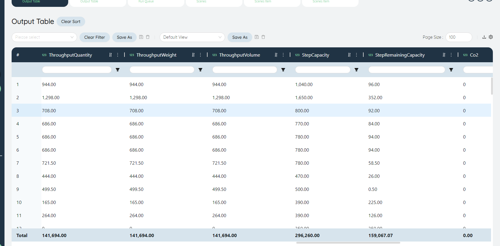
- OutputWorkCenterSummary
Displays the ThroughputLevel, ProductionCost, capacity utilization and other information of each production line in each Periods.
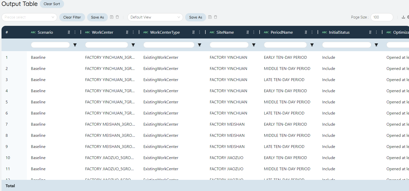
Optimize Status
According to FixedOperatingCost of WorkCenters, the capacity of the production line is located in which ladder.
ThroughputLevel/ThroughputLevel benchmark
According to the ConstraintValue benchmark field set in the input table-WorkCenters table, the ThroughputLevel benchmark is Hour.
ThroughputLevel under this Scenario represents the production schedule SnapshotDate of each production line in each tenth.
TotalCost
Under this Scenario is ProductionCost.
Throughput Quantity
Under this scenario, the Products Quantity actually produced by each production line every ten days is obtained according to ThroughputLevel (production SnapshotDate)*UnitProcessHour.
StepCapacity/StepCapacityRemaining/StepCapacityUtilization
In this Scenario, StepCapacity is the upper limit of the capacity of the capacity ladder where the production line is located, which comes from the upper limit of ThroughputLevel of the FixedOperatingCost field set in the input table - WorkCenters Multiple Periods.
StepCapacity Remaining = StepCapacity-Throughput Quantity.
StepCapacityUtilization=(StepCapacity-StepCapacity remaining)/StepCapacity.
TotalCapacity/TotalCapacity Remaining/TotalCapacityUtilization
Under this Scenario, there is only one step in capacity, TotalCapacity=StepCapacity.
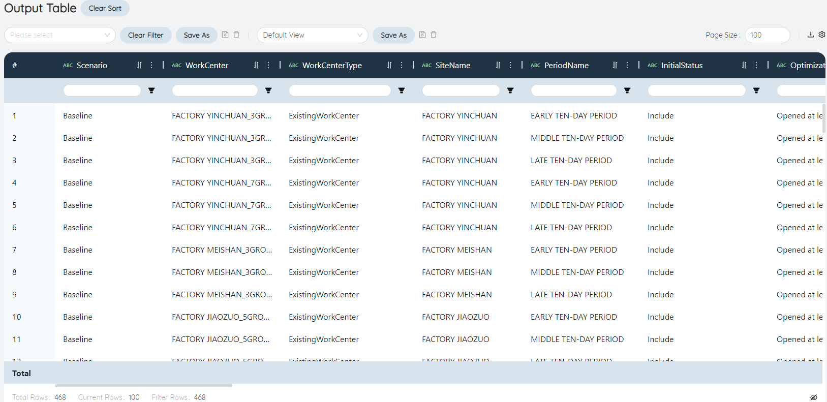
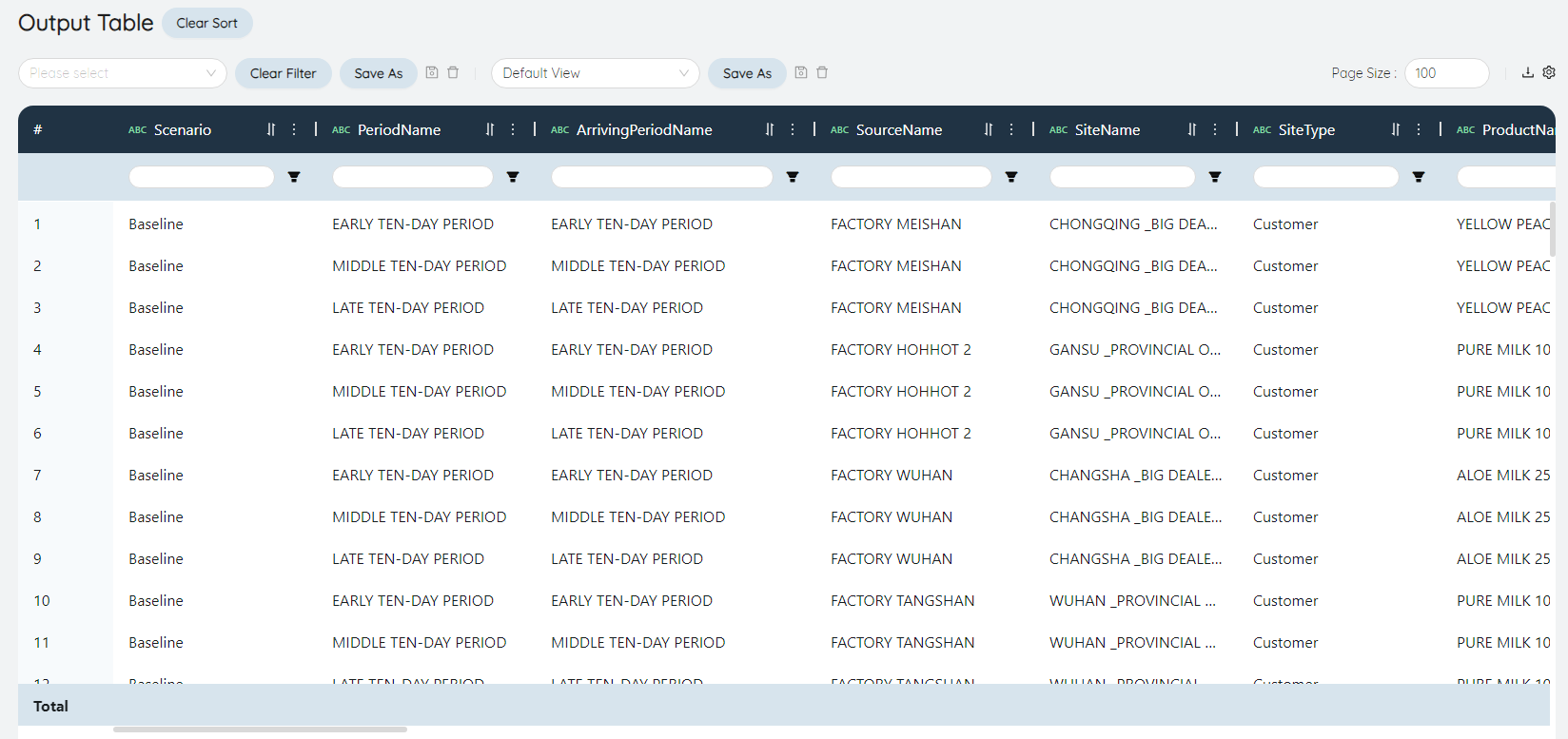
- Flow Details
On the basis of the ordinary Flow Details table, it also includes the Quantity and cost information of each Periods and each Sites discarded Products (finished products & raw materials).
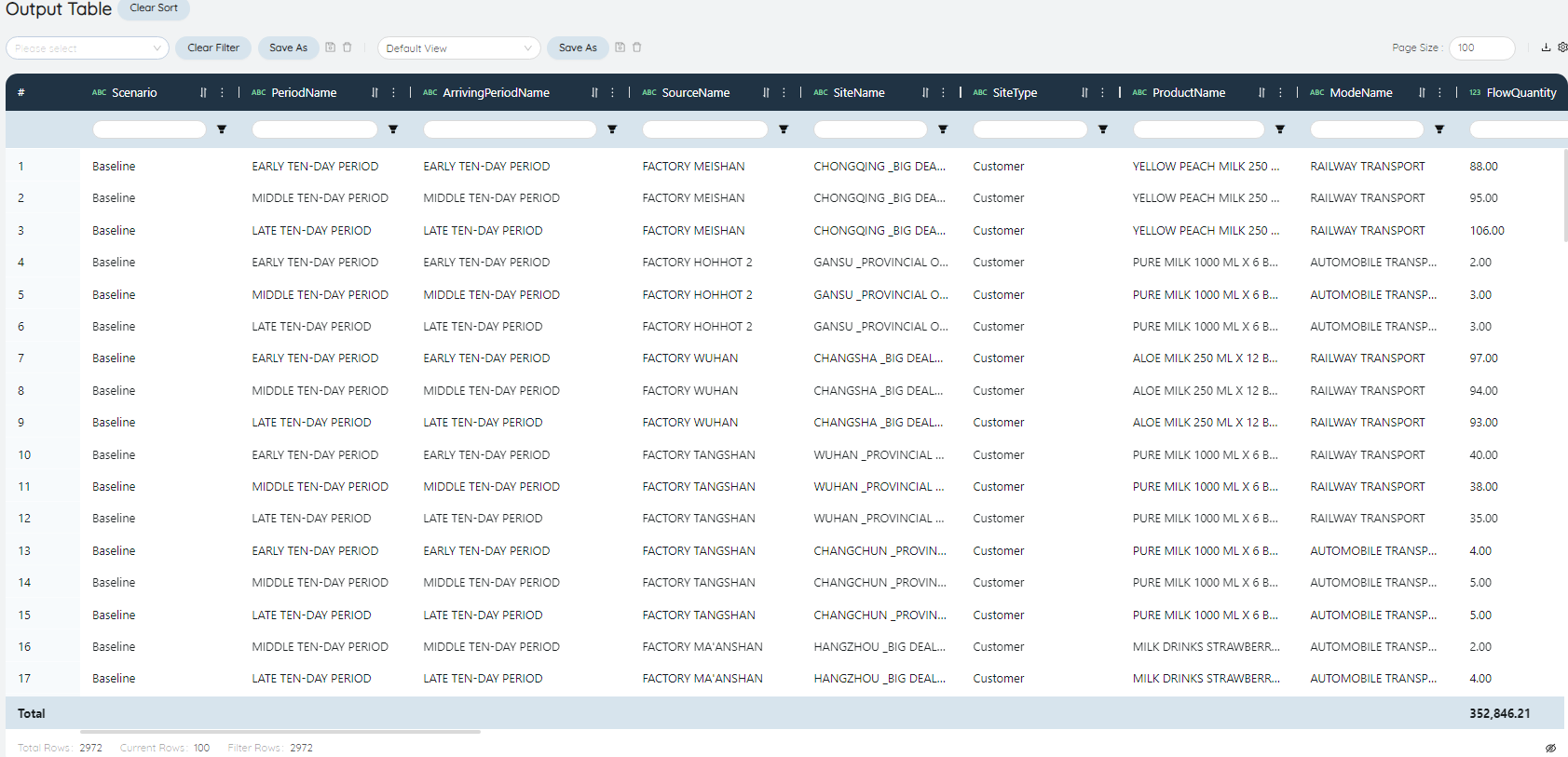
TransportModeName
In addition to the Transport ModeName involved in TransportationPolicies, there is also DISPOSAL , which means discard.
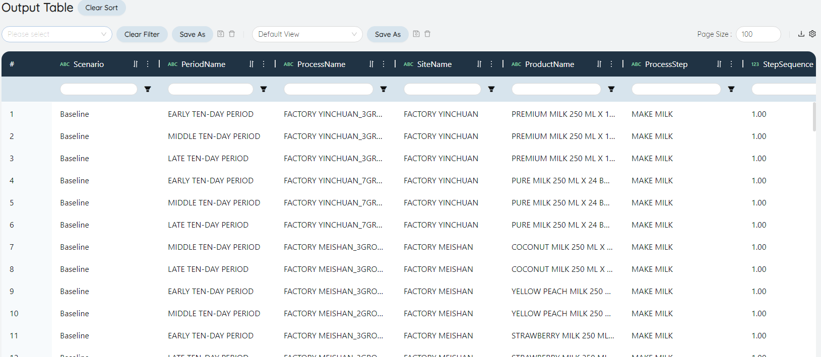
- OutputProduction
Displays the Quantity and cost breakdown information of each Product produced by each Periods and each Sites.

TotalProductionCost
Including ProductionCost formulated in ProductionPolicies and process cost formulated in ProductionProcess. Under this Scenario, equals the ProductionProcess cost.
# How to formulate optimization scenarios and predict optimization results? Build Scenario.
Lanxing Consultant gave the optimized Scenario of LX Milk:
- InitialInventory, raw milk production and CustomerOrders volume remain the same
- Lifting restrictions on production and distribution of finished products:
- Optimizing Scenario includes all possible routes and production plants in the input data, no longer restricts the type and Quantity of products produced by each plant, and the model comprehensively considers it according to the cost;
- Optimize the capacity limit of each production line in Scenario to remain unchanged;
- In the optimization Scenario, there is no longer a limit on the flow of Products per ten-day branch line, and the model will comprehensively consider it according to the cost.
To formulate and optimize the Scenario and build the Scenario, you first need to modify the input table: Add ProductionPolicies for all Products produced by the factory, and Purchase/TransportationPolicies with transportation quotations from the factory to the customer. Since InventoryPolicies is already available for all factories and can store all Products, there is no need to modify them. In the FlowConstraints table, add the FlowConstraints that are transmitted from the Dummy factory to each factory every ten days according to the Flow Details table output by the Baseline. Note that the Status is set to Exclude when modifying, otherwise it will affect the input of the Baseline; then you can start to build the Scenario, close the original FlowConstraints, open The newly added FlowConstraints from the Dummy factory to each factory , open the new production/purchasing/TransportationPolicies; after the optimization Scenario is set, the last key is to run NO to predict the optimization result.
# Model input
- ProductionPolicies

Add two ProductionPolicies as shown in the picture, so that the factory can produce all kinds of Products (finished products).
Note: Status is set to Exclude, and Notes is filled in to optimize Scenario.
- FlowConstraints
As shown in the picture, add FlowConstraints to lock the InitialInventory Quantity of each Product in each factory.
Note: Status is set to Exclude, and Notes is filled in to optimize Scenario.
- Scenario build
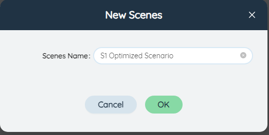
New Scenario: S1 Optimized Scenario
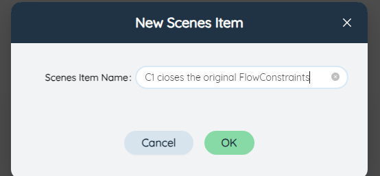
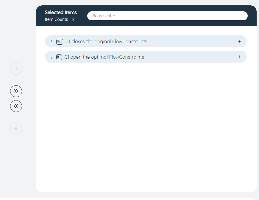
New Scenario item: C1 close the original FlowConstraints
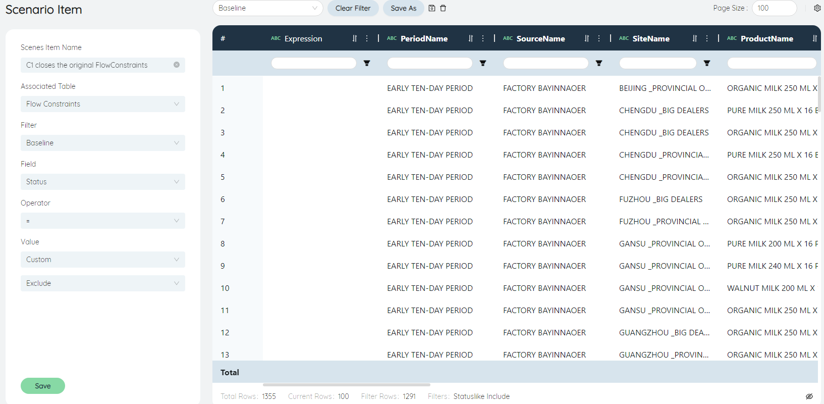
According to the picture prompt, filter Status as include, save the filter as Baseline, and modify the Status field=Exclude.
Click Save.
New Scenario item: C1 opens the optimal FlowConstraints
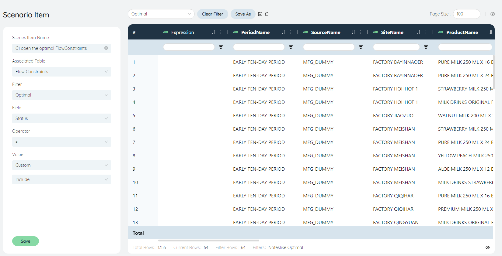
Similar to the previous Scenario item, the Notes are filtered to optimize the Scenario data, and the Status is changed to include.
Click Save.
Add both Scenario items to the Scenario.
# Model output
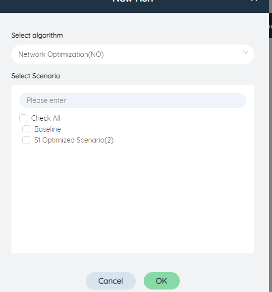
On the Online Task List menu, click Add Task to create an online task. Algorithm select Network Optimization (NO) algorithm, Scenario select S1 to optimize Scenario (2), click Add.
- OutputNetworkSummary

- OutputWorkCenterSummary
- Flow Details
- OutputProduction
# Scenario analysis and comparison
Perform data analysis on OutputNetworkSummary, OutputWorkCenterSummary, Flow Details table, and production flow table exported from SCATLAS.
Including comparative analysis of TotalCost, production and transportation before and after optimization.
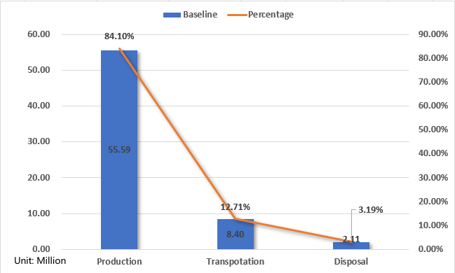
# Comparison of network costs before and after optimization
Baseline network cost structure
Optimized network cost composition
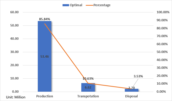
TotalDemand and InitialInventory remain unchanged.
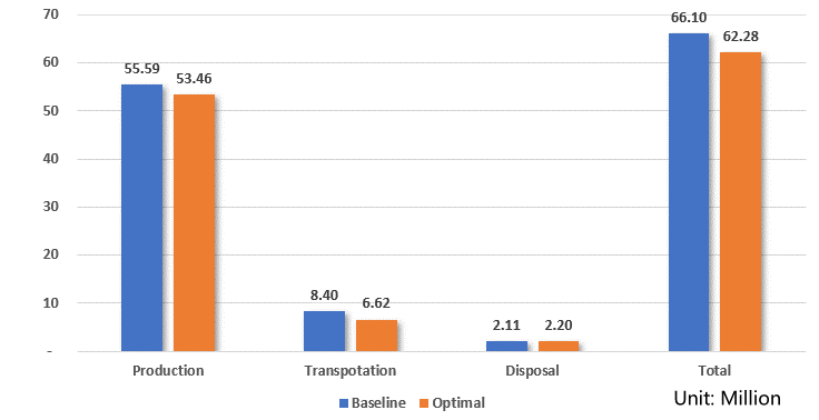
TotalProductionCost: After optimization, it decreased by 3.84%, about 2,136,146 yuan;
TotalTransportationCost: After optimization, it decreased by 21.23%, about 1,783,566 yuan;
Total discard cost: increased by 4.51% after optimization, about 95,030 yuan;
Total cost: decreased by 5.79% after optimization, about 3,824,683 yuan.
# Comparison of production before and after optimization
Different factories produce the same Product with different VariableCost and raw milk consumption. The TotalProductionCost and total raw milk consumption change slightly before and after optimization.
Average ProductionCost for each Product before and after optimization
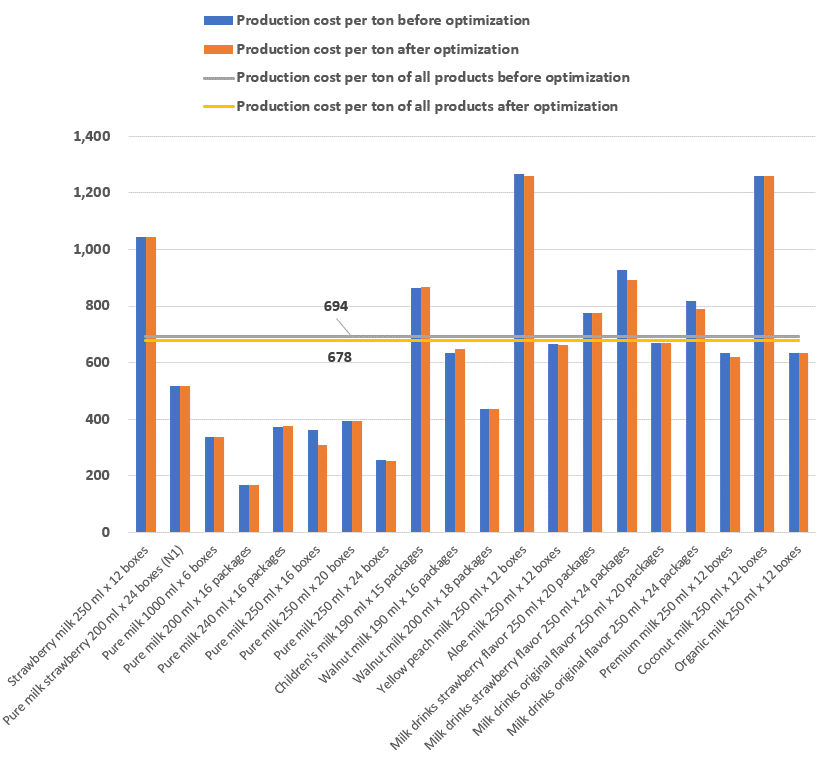
Summarize production Quantity and cost per ton before and after optimization by ten days
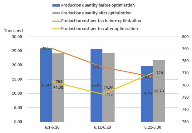
The average ProductionCost per ton of all Products before and after optimization decreased from ¥694 to ¥678.
After optimization, the production Quantity and VariableCost in the first half of the first ten days decreased, and the production Quantity and VariableCost in the latter half of the year increased.
After optimization, TotalProductionCost is reduced by 3.84%.
The number of production lines started in each ten-day period by capacity utilization before and after optimization
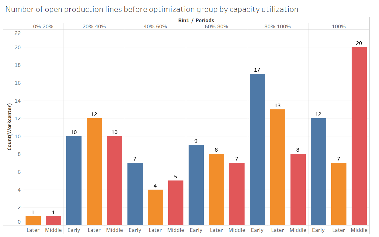
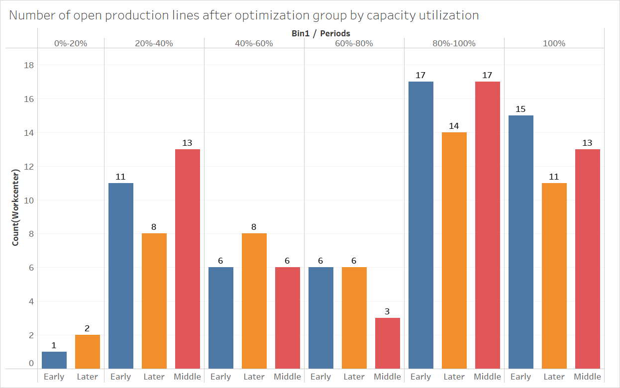
There are 56 production lines that started before optimization (utilization rate > 0) in the first ten days, 52 in the middle and 49 in the latter ten days.
There were 55 production lines that started operation after optimization (utilization rate > 0) in the first ten days, 51 in the middle and 45 in the latter ten days.
Average capacity utilization of production lines before and after optimization
The average capacity utilization rate of production lines whose utilization rate is greater than 0 per ten-day is better than that before optimization.
# Comparison of transportation situation before and after optimization
Optimized TransportationCost subdivision
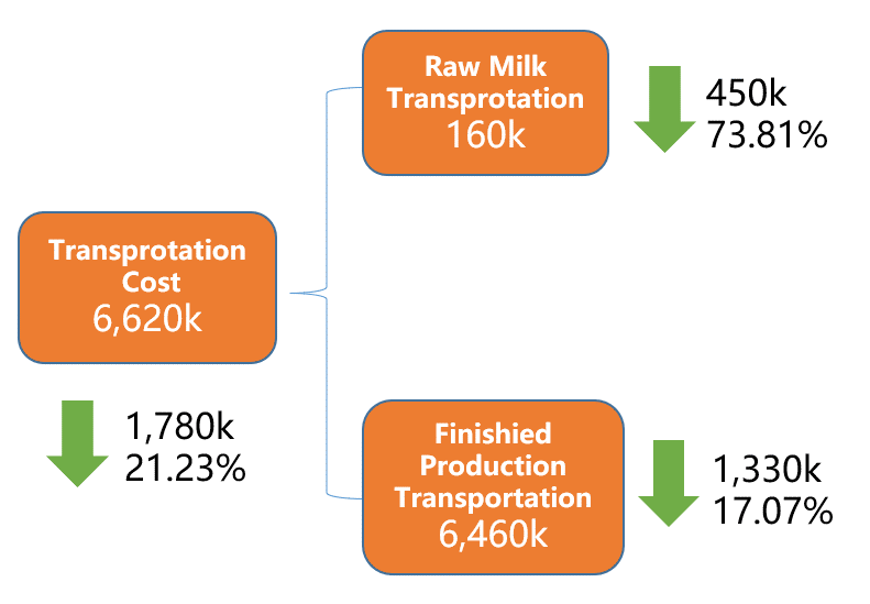
Comparison of raw milk allocation and shipping costs before and after optimization

After optimization, the amount of raw milk allocated is reduced, the total production volume remains unchanged, the total consumption of raw milk is basically unchanged, and the allocation of raw milk from different places is reduced.
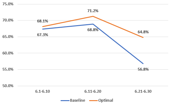
Comparison of the average distance and shipping cost of finished product distribution before and after optimization
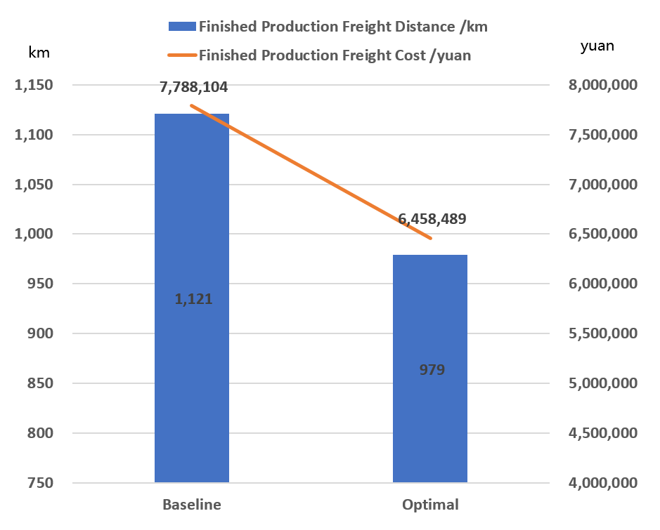
The TotalDemand remains unchanged, and the total freight is reduced. After optimization, customers are delivered by factories with closer distances. After optimization, the average delivery Distance is reduced, and customer ServiceHour is improved.
Comparison of transportation volume before and after optimization by transportation ModeName (tons)

Comparison of TransportationCost before and after optimization by transportation ModeName
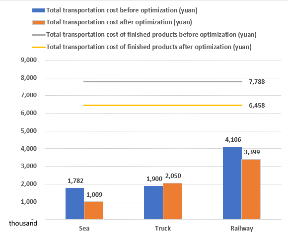
The total amount and cost of rail and sea transportation of finished product transportation decreased, and the total amount and cost of automobile transportation increased.